Adaptive Filtering in Electricity Spot Price Models

Shin Ichi Aihara

and Arunabha Bagchi

Department of Computer Media, Tokyo University of Science Suwa, 5000-1 Toyohira, Chino, Nagano, Japan

Department of Applied Mathematics, Twente University, P.O.Box 217, 7500AE, Ensched, The Netherlands

Keywords:

Electricity Spot, Risk premium, Hyperbolic system, Kalman ﬁlter, Jump process, Parameter identiﬁcation,

Parallel ﬁlter.

Abstract:

We study the adaptive ﬁltering for risk premium and system parameters in electricity futures modes. Introduc-

ing the jump augmented Vasicek model as the spot price mode, the factor model of the electricity futures is

constructed as the stochastic hyperbolic systems with jumps. Representing the main spike phenomena of the

electricity spot price from one observed futures data by proxy, the ﬁltering of the stochastic risk premium and

its system parameters are developed in a Gaussian framework. By using the parallel ﬁltering algorithm, the

online system parameter estimation procedure is proposed.

1 INTRODUCTION

It is well known that the electricity is quoted same

as any other commodity, e.g. crude oil, gold, copper

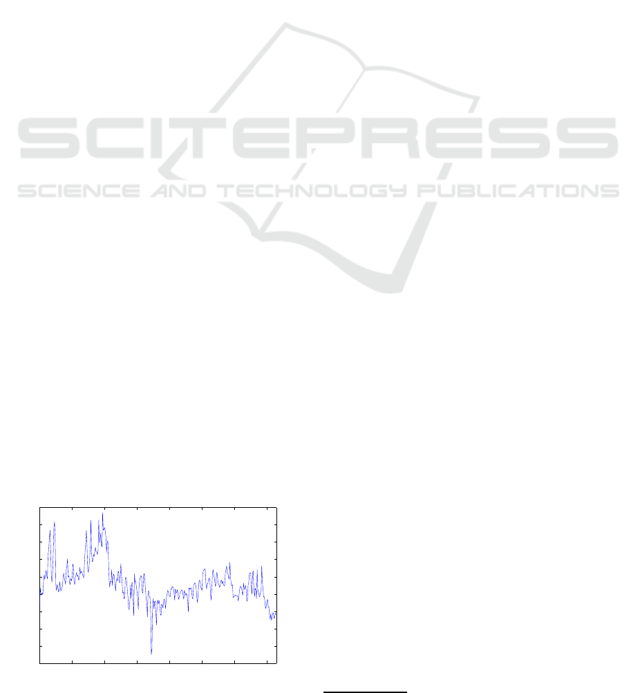
and others. As shown in Fig. 1, the electricity spot

prices present a higher volatility than equity prices

and its mathematical model is required for pricing of

electricity-related options, risk management and oth-

ers.

The peculiar characteristic of electricity is that one

can not store electricity, but there are many other char-

acteristics which distinguish electricity from other

commodities.

From Fig. 1, in which the spot price (a day-ahead

market) is shown, we observe the special behaviors

of electricity spot, i.e., many spikes frequently and

seasonal effect.

0 50 100 150 200 250 300 350

Time (day from 01/01/2013 to 31/12/2013)

Nord pool spot (EUR/MWh)

Figure 1: Nord Pool electricity spot price (day ahead im-

plicit auction market).

In this paper, instead of modeling this process

from the basic principle of supply and demand, the

simple mathematical model for this spot price is pro-

posed and leads to calibrate the model parameters

and price the options by using the stochastic sys-

tem approach. Along this line Schwartz and Smith

(Schwartz and Smith, 2000) proposed a two-factor

diffusion model and the system parameters are esti-

mated from M.L.E. (Maximum likelihood estimate)

by using Kalman ﬁlter. To apply this method one need

to add ad hoc observation noise in order to derive the

Kalman ﬁlter. This assumption has been made by nu-

merous authors, either in the commodity or interest

rate markets. The additional noise in the observa-

tion has been interpreted to bring into account bid-ask

spread, price limits or errors in the information. The

argument is clearly forced and unconvincing. By us-

ing the idea proposed by (Aihara and Bagchi, 2010),

we approach the modeling differently. In our setup,

on the one hand, the added measurement noise is

built in the model. On the other hand, the model-

ing of the correlation structure between the futures

(observation) is a natural component of our formu-

lation. Hence the model parameters can be calibrated

through the derived likelihood functional without any

ad hoc observation noise.

All the same, in these works, the important spikes

in the electricity prices could not be admitted, because

including jumps

means giving up on the closed-form

estimator like Kalman ﬁlter in (van Schuppen, 1977).

The closed-form formulae for forwards and options are

620

Aihara S. and BAGCHI A..

Adaptive Filtering in Electricity Spot Price Models.

DOI: 10.5220/0005014206200628

In Proceedings of the 11th International Conference on Informatics in Control, Automation and Robotics (ICINCO-2014), pages 620-628

ISBN: 978-989-758-039-0

 2014 SCITEPRESS (Science and Technology Publications, Lda.)

Fortunately, for the term structure model in the elec-

tricity problem, we can represent the jump process for

the spike phenomena by using one observation com-

ponent and transform the Non-Gaussian estimation

problem into the Gaussian framework with correlated

noises.

In this paper, from the real data (Nord Pool elec-

tricity spot data ), the linear trend is ﬁrstly identiﬁed

by using a least squares method. After subtracting this

linear trend from the spot data and taking the FFT, the

prominent frequencyof the seasonality effect is inves-

tigated in Sec.2. We choose the spot price dynamics

as the jump-diffusionmodel proposed in (Dufﬁeet al.,

2000). According to the idea in (Aihara and Bagchi,

2010), we construct the arbitrary free model of the

term structure, including jump-diffusion processes in

Sec.3. In the electricity market, the averaged-typefor-

ward and futures contracts are observed and are used

as the observation data for calibrating system param-

eters. After presenting this observation dynamics in

Sec.4, we derive the closed form ﬁlter for estimat-

ing the whole term structure. To derive this ﬁlter, we

choose one component of observation as the proxy for

the spike process of the spot price, say y

(t). Recon-

structing the spikes from y

(t) and plugging this into

observation and system equations, the ﬁltering prob-

lem with jumps is converted to the Gaussian frame-

work in Sec.5. For ﬁguring out the ﬁltering problem,

we need to work under the real world measure. Hence

a suggested in (Carmona and Ludkovski, 2004), the

stochastic market price of risk is introduced as the lin-

ear Ito equation. This implies that our extended state,

including the stochastic market price of risk is still

Gaussian. Instead of the use of MLE, we suggest the

parallel ﬁltering procedure in (Anderson and Moore,

1979) for obtaining the online state and parameter es-

timation. In the ﬁnal section, some numerical exam-

ples are demonstrated.

2 IDENTIFICATION OF LINEAR

TREND AND SEASONALITY

2.1 Linear Trend

From Fig.1, we can observe a slight downward trend

in the spot data in 2013. A least squares ﬁt gives the

trend line for the log price,

−6× 10

−4

t + 3.74.

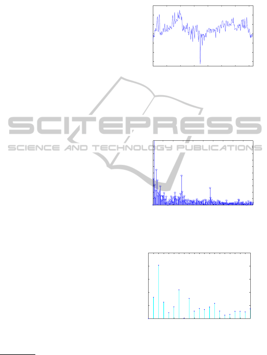
Now we subtract off this linear trend from the data

shown in Fig.1 and obtain the data shown in Fig.2.

possible, even for the jump-diffusion and Levy processes in

(Benth et al., 2008).

0 50 100 150 200 250 300 350

2.8

3.2

3.4

3.6

3.8

day

log S(t)− trend

Figure 2: Log price (day ahead implicit auction market) mi-

nus the linear trend.

2.2 Seasonality

We take the FFT to the data shown in Fig.2 and obtain

the periodogram shown in Fig.3. From Fig.3, we can

0 0.05 0.1 0.15 0.2 0.25 0.3 0.35 0.4 0.45 0.5

Real magnutude

Frequency[Hertz

Figure 3: Periodogram of the log spot.

ﬁnd big power points and zoom in on the plot and use

the reciprocal of frequency to label the x-axis in Fig.4.

365.0 182.5 121.7 91.2 73.0 60.8 52.1 45.6 40.6 36.5 33.2 30.4 28.1 26.1 24.3 22.8 21.5 20.3 19.2 18.2

days/cycle

power

Periodogram detail

Figure 4: Detail of periodogram.

The 365 days/cycle is not important, but we ﬁnd

still three outstanding points; 182.5, 60.8 and 45.6

days/cycle. We also need to ﬁnd phases at these points

(Red marks) in Fig.5.

AdaptiveFilteringinElectricitySpotPriceModels

621

0 0.05 0.1 0.15 0.2 0.25 0.3 0.35 0.4 0.45 0.5

−3

−2

−1

Angle

Frequency[Hertz

Figure 5: Angles at each frequencies.

Hence we ﬁnd that

Se(t) = Linear trend + Seasonality

= −6× 10

−4

t + 3.74

cos(2π × 16.4 × 10

−3

t − 2.8)

cos(2π × 142.5 × 10

−3

t − 0.05)

cos(2π × 284.9 × 10

−3

t + 2.11)(1)

The coefﬁcients a

and a

are identiﬁed to mini-

mize the |logS(t) − Seasonality - linear trend|

, i.e.,

= 0.114,a

= 0.006,a

= 0.042.

In Fig.6, we summarize the above results.

0 50 100 150 200 250 300 350

2.8

3.2

3.4

3.6

3.8

day

log S(t) − linear trend + 3.74

Seasonality

Log spot price − trend − seasonality

Log spot price − trend

Figure 6: Log price (day ahead implicit auction market)

with linear trend and seasonality.

3 SPOT RATE MODEL WITH

JUMPS

The spot price S(t) is set as

S(t) = exp(r(t)+ Se(t))

where Se(t) is identiﬁed by (1) and the short rate r(t)

is given by the jump augmented Vasicek model;

dr(t) = κ(¯r− r(t))dt + σ

(t) +

νp(dν, dt), (2)

where w

is a standard Brownian motion process

which is independent of the Poisson random measure

p and the compensated Poisson measure q

is is given

(dν, dt) = p(dν,dt) − (λ

(dν) + λ

−

(dν))dt

and where λ

(λ

−

) denotes the positive jump ( neg-

ative jump) time intensity and ψ

(ψ

) is a distribu-

tion of the positive (negative) jump size. In this paper

we more specify this jump process as the compound

Poisson processes:

νp(dν, dt) = J

(t;ψ

)dN(t;λ

)

(t;ψ

)dN(t;λ

−

where J

(t;ψ

) denotes the jump size with identically

distributed law ψ

and N(t,λ

) is a counting process

with parameter λ

. Here we shall present the simula-

tion results for these compounded Poisson processes:

0 0.2 0.4 0.6 0.8 1

−1.5

−1

−0.5

0.5

1.5

Time

Compound Poisson

Figure 7: Compounded Poisson process.

4 ELECTRICITY MODEL

By a basic no-arbitrage argument it follows that the

price of a futures contract F(t, T −t) which has payoff

S(T) at future time T equals to

F(t,T − t) = E{S(T)|F

with respect to the risk neutral measure. Hence we

can write the futures price as

F(t, T − t) = exp{A(t, T − t)+ B(t,T − t)r(t)}, (3)

where A and B satisfy deterministic equations. (See in

(Dufﬁe et al., 2000) for details.) Although this model

ICINCO2014-11thInternationalConferenceonInformaticsinControl,AutomationandRobotics

622

is mathematically elegant, it is not consistent with the

forward curve as stated in (Carmona and Ludkovski,

2004). From the systems identiﬁcation view points,

the observation futures data are summed to the artiﬁ-

cial observation noises. In order to avoid this ambigu-

ity, we append the extra noise in (3) as used in (Aihara

and Bagchi, 2010). This noise represents the model

errors from the basic property of r(t). This will mean

that the corresponding futures price should be given

by a slight perturbation of (3),i.e.,

F(t, T − t) = exp{A(t, T − t) + B(t,T −t)r(t)

σdw(s, T − s)}, (4)

where we use the same symbols in (3) and

σdw(s, T − s) =

∞

∑

k=1

(T − s)dβ

(s), (5)

and where e

(·) is a sequence of differentiable func-

tions forming an orthonormal basis in L

(0,T

∗

)

and

{β

(t)} are mutually independent Brownian motion

processes with

∑

< ∞,i.e.,

E{w(t,x

)w(t,x

)} = tq(x

)

and

∗

q(x,x)dx =

∞

∑

k=1

< ∞.

Setting

f(t,x) = A(t,x) + B(x)r(t)+

σdw(s, x+ t − s), (6)

the futures contracts F(t,T − t) becomes

F(t, T − t) = exp( f(t,T − t)) (7)

with F(T,0) = exp( f(T, 0)) = S(T). Now we derive

the explicit forms of A and B so that F(t,T − t) is a

martingale in the risk neutral measure. Applying

the results by (Aihara and Bagchi, 2010), we get The

explicit form of (6) is a solution of

d f(t, x) =

∂f(t,x)

∂x

dt − ˜q

(x)dt + e

−κx

{σ

(t)

νq

(dν, dt)} + σdw(t,x) (8)

f(0,x) = ¯r(1− e

−κx

) +

2κ

(1− e

−2κx

)

q(z,z)dz+ Se(x) + e

−κx

r(0)

(λ

(z) + λ

−

(z))dz, (9)

∗

denotes the longest future time in mind

where

˜q

(x) = σ

−2κx

q(x,x) + (λ

(x) + λ

−

(x))

and

•

(x) =

exp(e

−κx

ν)ψ

•

(dν) − 1. (10)

5 REAL WORLD DYNAMICS

On the identiﬁcation problem, we work in the real

world measure. For example, we add a simple risk

premium term to (8) . In this paper, we simplify the

position that the market price of risk Λ

(t) comes

mainly from w

(t) but this moves stochastically. We

set this term as

dΛ

(t) = κ

(

Λ− Λ

(t))dt + σ

(t), (11)

where the BMP w

is independent of w

. Now under

the real world measure the BMP ˜w

(t) is represented

(t) = ˜w

(t) −

(s)ds.

Hence our system state [f(t, x) Λ

(t)] under the phys-

ical measure becomes











d f(t, x) =

∂f(t,x)

∂x

dt − ˜q

(x)dt

−κx

{σ

(−Λ

(t)dt

+d ˜w

(t)) +

νq

(dν, dt)} + σdw(t,x)

dΛ

(t) = κ

(

Λ− Λ

(t))dt + σ

(t).

(12)

6 OBSERVATION

Noting that electricity is essentially not storable, the

futures contracts are based on the arithmetic averages

of the spot prices over a delivery period [T

,T], given

T − T

S(τ)dτ.

Now, for t < T

we can calculate the futures prices by

F(t, T

,T) = E{

T − T

S(τ)dτ|S(t)}

T − T

F(τ,t)dτ

T − T

T−t

−t

exp[ f(t,x)]dx. (13)

In practice we adopt the geometric average as an ap-

proximation;

F(t,T

,T) ∼ exp[

T − T

T−t

−t

f(t,x)dx]. (14)

AdaptiveFilteringinElectricitySpotPriceModels

623

By using this geometric approximation, the observa-

tion data for the futures price is set as

(t) =

T − T

+(T−T

)

f(t,x)dx, (15)

where τ

< τ

< ··· < τ

Denoting

Y(t) = [y

(t)]

m×1

we have

Y(t) = H

f(t,·)dt − H( ˜q

+ B(x)σ

(t))dt

+H[dw

(t,·)] + H[B

νq

(dν, dt)], (16)

where B(x) = e

−κx

(t,x) = B(x)σ

(t) + σw(t,x), (17)

H(·) =

T − T

[

+(T−T

)

(·)dx, · · · ,

+(T−T

)

(·)dx]

′

and

(·) = [

T − T

(δ(η− (T − T

+ τ

))

− δ(η− τ

))(·)dη]

m×1

6.1 Reconstruction of Jump Process

Choosing one yield data for τ

< τ

(t) =

T − T

+(T−T

)

f(t,x)dx, (18)

we have

(t) = H

f(t,·)dt − H

( ˜q

+ B(x)σ

(t))dt

[dw

(t,·)] + H

νq

(dν, dt)],

where H

(·) =

T−T

+(T−T

)

(·)dx, and

(·) =

T − T

(δ(η− (T − T

+ τ

))

−δ(η− τ

))(·)dη.

Hence it is possible to reconstruct the jump pro-

cess from y

(t) such that

νq

(dν, ds)

(t) −

fds− H

(t,x))

( ˜q

+ B(x)σ

(s))ds, (19)

where B

= H

B. Plugging (19) into (12), we have

d f(t, x) =

∂f(t,x)

∂x

dt − ( ˜q

(x) + B(x)σ

(t))dt

+dw

(t,x) +

B(x)

{dy

(t) − H

fdt

( ˜q

+ B(x)σ

(t))dt − H

(t,x)} .(20)

We transform the above equation as the robust form

for jump term. Deﬁne

f(t, x) = f(t, x) −

B(x)

(t). (21)

Hence we get

f(t,x) = (

∂

∂x

− C

)(

f(t, x) +

B(x)

(t))dt

−(1− C

)( ˜q

(x) + B(x)σ

(t))dt

+ (1− C

)σdw(t,x), (22)

where

B(x)

, C

B(x)

. (23)

6.2 Reconstruction of Observed Yields

The original yield y

(t) becomes

(t) = H

f(t,·)

= H

f(t,·) +

(t). (24)

Now we construct the new observation such that

˜y

(t) = y

(t) −

(t),

= H

f(t, ·). (25)

Denoting

Y(t) = [ ˜y

(t)]

m×1

and from (H − HC

)Bσ

= HBσ

−HBσ

0, we get

Y(t) = (H

− HC

)

f(t, ·)dt + (H

− HC

)

(t)dt − (H−HC

) ˜q

dt + (H − HC

)σdw(t,x).

(26)

We ued w

−

= (1−

)σw.

We used H

(·) =

(T−T

)

+(T−T

)

(·)dx.

ICINCO2014-11thInternationalConferenceonInformaticsinControl,AutomationandRobotics

624

7 THE KALMAN FILTER

In (8), Poisson jump processes are included and this

is not a usual Kalman ﬁlter problem. There are many

articles for Non-Gaussian ﬁltering problem by using a

martingale approach, e.g. (van Schuppen, 1977) and

however it is still difﬁcult to derive the closed form

ﬁltering algorithm. In our position, the transformed

system (22) with the observation (26) do not include

jump processes explicitly. Hence our estimation prob-

lem is in the Gaussian framework;



f(t,x)

(t)





(

∂

∂x

− C

) − (1−C

)

0− κ



f(t,x)

(t)





(

∂

∂x

− C

)

− (1− C

) ˜q



+ d



(1− C

)w(t, x)

(t)



. (27)

with

Y(t) = (H

− HC

,0)



f(t,x)

(t)



+((H

− HC

)

(t) − (H − HC

) ˜q

)dt

+(H − HC

)dw(t,x). (28)

Denoting ˆ· = E{·|Y

}, for Y

= σ{

Y(s),y

(s);0 ≤

s ≤ t}, we have

f(t,x) = (

∂

∂x

− C

)(

f(t, x) +

B(x)

(t))dt

−(1− C

)(B(x)

(t) + ˜q

(x))dt



f f

(t)(H

− HC

)

∗

+(1− C

)Q(H − HC

)

∗

}

−1

(

Y(t) − (H

− HC

,0)

f(t,x)

(t)

−((H

− HC

)

(t) − (H − HC

) ˜q



,(29)

and

(t) = κ

(

Λ−

(t)dt

Λf

(t)(H

− HC

)

∗

−1

(

Y(t)− (H

− HC

,0)

f(t, x)

(t)

−((H

− HC

)

(t) + (H − HC

) ˜q



,(30)

where Q =

q(x,z)(·)dz ,

Φ = (H − HC

)((H − HC

)Q)

∗

, (31)

and

∂

f f

(t)

∂t

= (

∂

∂x

− C

)

f f

(t) +

f f

(t)(

∂

∂x

− C

)

∗

−

fΛ

(1− C

)

∗

− (1− C

)

Λ f

+ (1− C

)Q(1− C

)

∗

−



f f

(t)(H

−

)

∗

+ (1− C

)Q(H − HC

)

∗



−1



f f

(t)(H

−

)

∗

+ (1− C

)Q(H − HC

)

∗



∗

(32)

∂

fΛ

(t)

∂t

= (

∂

∂x

− C

)

fΛ

(t) −

fΛ

(t)κ

−



f f

(t)(H

−

)

∗

+ (1− C

)Q(H − HC

)

∗



−1



Λ f

(t)(H

−

)

∗



∗

(33)

8 ADAPTIVE FILTERING

PROBLEM

8.1 Parallel Filtering

To construct the parameter estimation algorithm, we

conﬁne the general jump process as the compound

Poisson process as stated in Remark, i.e., J

(t;φ

) =

Gaussian with mean m

and variance σ

and i.i.d for

each jump time and same as the negativejump. Hence

we have

(x) = exp[

B(y)dy(m

(σ

)

)].

As used in (Aihara and Bagchi, 2010), we set the

function form q(x, x). Hence the unknown system pa-

rameters

θ = [κ ¯r σ σ

−

Λ σ

] ∈ Θ ⊂ R

where Θ is a known bounded set. Following from

(Anderson and Moore, 1979), the following parallel

ﬁltering algorithm is made:

• Set candidates of unknown parameter θ such that

( j)

∈ uniform random vectors in Θ, j = 1, ·, ·, m

• For each θ

( j)

, we solve the Kalman ﬁlter (29, 30)

for t

≤ t ≤ t

i+1

r is estimated from the initial forward cure. See (Aihara

and Bagchi, 2010)

AdaptiveFilteringinElectricitySpotPriceModels

625

• Calculate the posteriori probability,

p(θ

( j)

Y(t

)

p(θ

( j)

Y(t

))p(

Y(t

i+1

)|θ

( j)

Y(t

))

∑

k=1

Y(t

i+1

)|θ

(k)

Y(t

))p(θ

(k)

Y(t

))

where

Y(t

i+1

)|θ

( j)

Y(t

)) ∝ exp



i+1

Y(s)

′

−1

(

Y(t)− (H

− HC

,0)

f(t,x)

(t)

−((H

− HC

)

(t) − (H − HC

) ˜q



• The estimates of f and θ are given by

f(t

i+1

,x) =

∑

i=1

f(t

i+1

,x;θ

( j)

)p(θ

( j)

Y(t

i+1

))

θ =

∑

i=1

( j)

p(θ

( j)

Y(t

i+1

)).

8.2 Resample Procedure for Parameters

The parallel ﬁlter algorithm is not sensitive for iden-

tifying many unknown parameters. In this paper, we

propose a new resampling procedure to increase the

diversity of parameter estimates.

• Set the resampling time period t

resamp

• At the time t

= (n−1)t

resamp

for n = 1,2, ···, cal-

culate

θ(i)

∑

j=1

{(θ

( j)

)

p(θ

( j)

Y(t

)) −

(i)}

for i = 1, 2, · · · , 12.

• Construct the posteriori distribution by using the

Gaussian approximation:

P(θ(i)|

Y(t

)) ∼ N (θ(i);

θ(i),ε

θ(i)

where ε denotes a user deﬁned parameter.

• Generate new samples θ

( j)

(i) in Θ from

P(θ(i)|

Y(t

)). To get new samples in Θ, we use

the systematic resampling procedure.

• Reset p(θ

( j)

Y(t

)) =

9 SIMULATION STUDIES

In this simulation study, we set the system parameters

in Table-1

Table 1: Systems parameters.

κ ¯r σ

σ m

, σ

5.00 3.00 0.80 0.1 0.30 8.00 0.20

−

Λ σ

-0.30 8.00 0.20 6.00 0.40 2.00

Setting the seasonality and linear trend functions

are set in Sec.2, we simulate (12) by using the ﬁ-

nite difference method with dx = 0.01, dt = 0.005 in

Fig.8.

We also generate the observation data

Y(t) =

[10y

(t)]

for i = 1,2, · · · , 7 with τ

= 0, τ

0.1, ··· , τ

= 0.6 shown in Fig.9.

0.2

0.4

0.5

2.5

3.5

4.5

Time(year)

Time−to−maturity

f(t, x)

Figure 8: f (t, x)- process.

0 0.1 0.2 0.3 0.4 0.5

0.24

0.26

0.28

0.3

0.32

0.34

0.36

Time(year)

Observation data y

Figure 9: Observed data

If all systems parameters are known, the Kalman

ﬁlter works good and such simulation results are

found in (Aihara et al., 2014). Here we shall look

into the feasibility of the proposed on-line algorithm.

Hence we set the upper and lower bounds for the un-

known parameters shown in Table-2 with the tuning

parameters ε

ICINCO2014-11thInternationalConferenceonInformaticsinControl,AutomationandRobotics

626

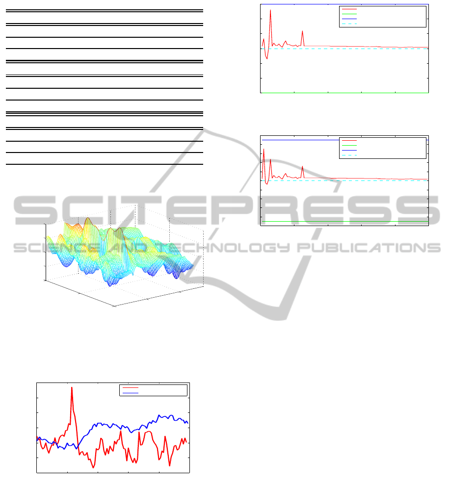
Table 2: Upper and lower bounds for systems parameters.

κ ¯r σ

σ m

Upper 6.5 3.9 1.04 0.13 0.39

Lower 3.5 2.1 0.56 0.07 0.21

1.05 1.05 1.05 1.05 1.05

−

Upper 10.4 0.26 -0.21 10.4.00 0.26

Lower 5.6 0.14 -0.39 5.6 0.14

1.05 1.05 1.05 1.05 1.05

Λ σ

Upper 7.8 0.52 2.6

Lower 4.2 0.28 1.4

1.05 1.05 1.05

The estimate

f(t,x) is shown in Fig. 10.

0.2

0.4

0.5

2.5

3.5

4.5

Time(year)

Time−to−maturity

f(t, x)

Figure 10: Estimated

f(t,x).

The estimate of the market price of risk is demon-

strated in Fig.11.

0 0.1 0.2 0.3 0.4 0.5

−2

−1

Time(year)

True and estimated Λ

Estimated

True Λ

Figure 11: True and estimated Λ

(t).

Now we call demonstrate the estimates of un-

known parameters where we selected for κ, and ¯r in

Figs.12 and 13. The estimates of other parameters

have almost same beavers in these images.

0 0.1 0.2 0.3 0.4 0.5

3.5

4.5

5.5

6.5

Time (year)

True and estimated parameters

Estimated value

Lower bound

Upper bound

True value

Figure 12: True and estimated κ.

0 0.1 0.2 0.3 0.4 0.5

2.2

2.4

2.6

2.8

3.2

3.4

3.6

3.8

Time (year)

True and estimated parameters

Estimated value

Lower bound

Upper bound

True value

Figure 13: True and estimated ¯r.

10 CONCLUSIONS

Bringing in the compound Poisson jump process, the

stochastic model for the electricity futures has been

suggested. By using the idea proposed by (Aihara

et al., 2014) the original ﬁltering problem is changed

to the Gaussian framework and its Kalman ﬁlter is de-

rived. In the adaptive ﬁltering algorithm, the parallel

ﬁltering method in (Anderson and Moore, 1979) is

used to obtain the on-line parameter estimates with

the new resampling procedure. From the proposed al-

gorithm, it is not possible to estimate the noise corre-

lation parameter, if it exits. The possible way to iden-

tify this parameter is to use the Rao-Blackwellized ﬁl-

ter.

REFERENCES

Aihara, S. and Bagchi, A. (2010). Identiﬁcation of afﬁne

term structures from yield curve data. International

Journal of Theoretical and Applied Finance, 13:27–

47.

Aihara, S., Bagchi, A., and Imreizeeq, E. (2014). Filtering

and identiﬁcation of stochastic risk premium for elec-

tricity spot price models. Proc. of 19th IFAC World

Congress, page to appear.

Anderson, B. and Moore, J. (1979). Optimal Filtering.

Prentice-Hall, Inc., Englewood Cliffs.

Benth, F.,

S. Benth, J., and Koekebakker, S. (2008).

AdaptiveFilteringinElectricitySpotPriceModels

627

Stochastic Modelling of Electricity and Related Mar-

kets. World Scientiﬁc, Singapore.

Carmona, R. and Ludkovski, M. (2004). Spot convenience

yield models for the energy markets. In Mathematics

of ﬁnance, volume 351 of Contemp. Math., pages 65–

79. Amer. Math. Soc., Providence, RI.

Dufﬁe, D., Pan, J., and Singleton, K. (2000). Transform

analysis and asset pricing fro afﬁne jump-diffusions.

Econometrica, 68(6):1343–1376.

Schwartz, E. and Smith, J. (2000). Short-term variations

and long-term dynamics in commodity prices. Man-

agement Science, 46/7:893–911.

van Schuppen, J. (1977). Filtering prediction and smooth-

ing for counting process observations, a martingale

approach. SIAM J. Appl. Math., 32-2:552–570.

ICINCO2014-11thInternationalConferenceonInformaticsinControl,AutomationandRobotics

628

REFERENCES

Aihara, S. and Bagchi, A. (2010). Identification of affine