
Simulation Validation of the Model-based Control of the Plate Heat
Exchanger with On-line Compensation for Modelling Inaccuracies
Michal Fratczak, Jacek Czeczot and Pawel Nowak
Silesian University of Technology, Faculty of Automatic Control, Electronics and Computer Science,
Institute of Automatic Control, Gliwice, Poland
Keywords: Distributed Parameter Modelling, Model-based Control, Plate Heat Exchangers, Linearizing Adaptive
Control, Simulation Validation.
Abstract: This paper describes the stage of initial validation of the model-based control of the plate heat exchanger
(PHE) by simulation. For the distributed parameter model of PHE validated on the basis of the measurement
data collected from the real process, the approximation by the orthogonal collocation method is applied and
then the linearizing controller with the on-line compensation for the potential modelling inaccuracies is
suggested. This approach ensures relatively low computational complexity due to the low dimension of the
approximating dynamical model, which allows for its practical implementation in the programmable logic
controllers. The suggested controller is tested by simulation under the realistic experiments scenario and it
shows its superiority and robustness over the conventional PI controller, for both tracking and disturbances
rejection. The results show that the suggested concept can be considered as an interesting model-based
alternative for the PID-based control systems that are still widely applied in the industrial practice.
1 INTRODUCTION
For last decades, the plate heat exchangers (PHE)
have become more and more popular in the
industrial and domestic heat exchange and
distribution networks, due to their compact
dimensions and very high heat transfer efficiency.
At the same time, the control of such units is still the
challenge due to their nonlinear dynamics, especially
because the modern industrial systems demand
growing improvement in product quality at possibly
lowest energy consumption and other operation
costs, combined with high safety and environmental
goals (Bauer and Craig, 2008).
Dynamical modelling of PHEs that would
account for their characteristic construction is more
complex in comparison to the conventional approach
based on tubular double-pipe approximation. In
literature, only few approaches to this problem can
be found - e.g. (Georgiadis and Macchietto, 2000;
Gut and Pinto, 2003). Based on the interaction
between the plates, the fundamental energy
conservation law is applied to derive a set of
approximating dynamical equations, describing the
variation of the temperatures in the cold and hot
zones.
This paper deals with the synthesis of the model-
based controller for PHEs and the intension is to
incorporate the nonlinearities and the complex
dynamics of such a unit into the resulting control
law. Thus, it is crucial to derive the model of
possibly lowest complexity that would be able to
describe the heat exchange process taking place in
PHE with possibly high accuracy and this goal
requires the distributed parameter modelling. Then,
such a model can be considered as a basis for
deriving the model-based controller.
This approach is very promising but in the
practice, there is always a problem resulting from
potential modelling inaccuracies. Any model-based
controller suffers from the limited accuracy of the
model and thus, one of the possible methods for the
inaccuracy compensation should be applied. One of
them is the application of the integral action, which
always ensures offset-free control but at the same
time, it introduces the inconvenient dynamics to the
control system. The examples of this approach for
the control of the tubular heat exchangers can be
found in (Maidi, Diaf and Corriou, 2009; 2010). The
other possibility is to compensate for the modelling
inaccuracies by the on-line adjustment of the chosen
model parameters, which represents the case of the
657
Fratczak M., Czeczot J. and Nowak P..
Simulation Validation of the Model-based Control of the Plate Heat Exchanger with On-line Compensation for Modelling Inaccuracies.
DOI: 10.5220/0005015006570665
In Proceedings of the 4th International Conference on Simulation and Modeling Methodologies, Technologies and Applications (SIMULTECH-2014),
pages 657-665
ISBN: 978-989-758-038-3
Copyright
c
2014 SCITEPRESS (Science and Technology Publications, Lda.)
nonstationary modelling with the on-line model
update. This possibility was studied for the tubular
flow reactors (Czeczot, 2003).
In this paper, it is suggested how the linearizing
control methodology (e.g. Isidori, 1989; Henson and
Seborg, 1997) can be applied to control PHE and
how the linearizing controller can be derived based
on its distributed parameter model. The lower
complexity of the model is ensured by applying the
tubular double-pipe approximation with the model
parameters optimally adjusted on the basis of the
measurement data collected from the PHE working
in the real heating system. This model is further
simplified by its space discretization by the
orthogonal collocation method (OCM) (Villadsen
and Michelsen, 1978), which ensures significantly
lower dimension of the approximating state vector.
Then, based on this simplified model, the linearizing
controller is derived and the compensation for
modelling inaccuracies is ensured without any
integral action in the resulting control law. The
suggested controller is finally tested by simulation
under the realistic experiments scenario in the
application to control the PHE modelled as the
complete distributed parameter system.
2 PROBLEM STATEMENT
In this work, the problem of the model-based control
of the counter-current PHE operating in the setup
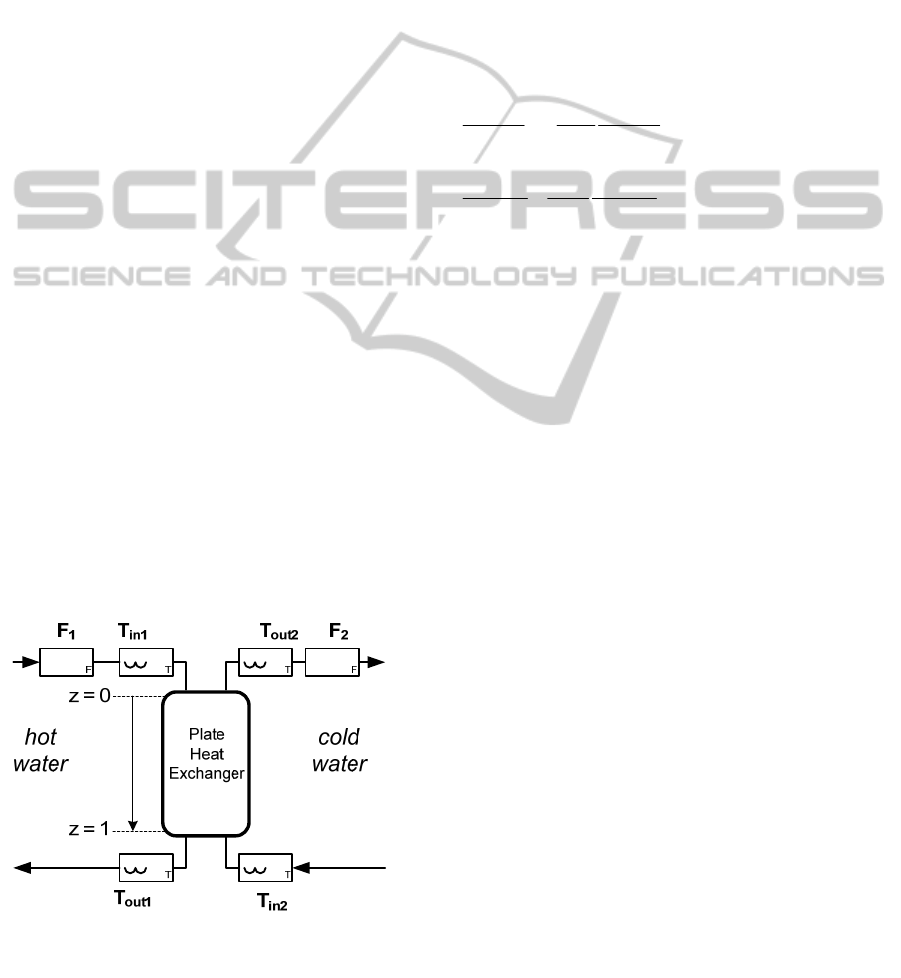
presented schematically in Fig. 1 is considered. It is
assumed that the unit is equipped with the sensors
for both flow rates F
1
, F
2
[L/min] and for inlet and
outlet temperatures T
in1
, T
in2
, T
out1
, T
out2
[
o
C],
respectively.
Figure 1: Schematic diagram of the considered PHE setup.
The control goal is defined to stabilize the outlet
temperature of the cold water Y = T
out2
by
manipulating the inlet temperature of the hot water
u = T
in1
. The flow rate of the hot water F
1
is assumed
to be adjustable and constant while the unit is
disturbed by the measurable variations of the inlet
temperature T
in2
and by the flow rate F
2
of the cold
water, which represent the variations of the heat
demand.
In this paper, the real PHE is described by the
simplified tubular double-pipe model based on the
energy balance and assuming perfect insulation of
the unit. This model consists of two partial
differential equations describing respectively the
temperatures of the hot water T
1
[
o
C] and of the cold
water T
2
[
o
C]:
),(),(
),()(),(
211
1
1
11
tzTtzTh
z
tzT
p
tF
t
tzT
(1a)
),(),(
),()(),(
212
2
2
22
tzTtzTh
z
tzT
p
tF
t
tzT
(1b)
with the boundary conditions:
)(),1(),(),0(
2211
tTtTtTtT
inin
,
(1c)
and the initial profiles )0,(),0,(
21
zTzT . At the same
time, the outlet temperatures are defined as
),0()(),,1()(
2211
tTtTtTtT
outout
, for the hot and
cold water, respectively.
In Eqs. (1), ∈
0,1
denotes the normalized
space variable, which makes the model independent
from the geometrical dimensions of the certain PHE
under consideration. For tubular heat exchangers,
the space variable is normalized as /, where
∈
0,
and L denotes the length of the tube.
However, readers should note that in the case of any
PHE, its geometrical length is not equivalent to the
substitute length of the channels between the plates
that usually is unknown. Thus, it was decided to
avoid this length in the model (1) and its influence is
lumped in the substitute geometrical parameters p
1
and p
2
. Two other model parameters h
1
and h
2
denote the substitute heat exchange coefficients.
During the simulation experiments, the model (1)
was solved numerically by the space discretization
finite difference method (FDM) (Carver and Hinds,
1978) with the constant space discretization instant
Δz = 0.02.
The suggested model (1) is the simplification
because its form does not match the construction of
the real PHE unit. However, this simplification is
fully justified if the parameters p
1
, p
2
, h
1
and h
2
were
assumed to be time-varying with the values
depending on the variations of the operating point of
the heat exchange process. In this work, their values
SIMULTECH2014-4thInternationalConferenceonSimulationandModelingMethodologies,Technologiesand
Applications
658

were indentified based on the measurement data
collected from the real PHE working as a part of the
laboratory heat exchange and distribution plant. The
experiments were carried out for different operating
points defined by different inlet temperatures and
flow rates in both circuits. Both flow rates F
1
, F
2
were successively adjusted within the range between
1.5 and 3.5 with the increment of 0.5, always
keeping the flow F
2
equal or smaller than the flow
rate F
1
. For each operating point, the variations of
the inlet temperature of the hot water T
in1
were
applied to the unit by the successive step changes of
the power supplied to the electric flow heater
warming the hot water flowing into PHE.
Based on the modelling error e = (T
out,P
- T
out,M
),
where T
out,P
represents the vector of the measured
values of T
out1
, T
out2
while T
out,M
represents the vector
of the corresponding temperatures computed from
the model (1) excited with the same measured input
signals, the following quality factor was defined:
eehhppJ
T
Q,,,,
2121
,
0diag qQ
(2)
and the optimal values of the parameters p
1
, p
2
, h
1
and h
2
were identified for each operating point by
the minimization of J(.) applying the Nelder and
Mead Simplex numerical algorithm (Nelder and
Mead, 1965; Lagarias, Reeds, Wright, and Wright,
1998). It was found that the optimal values of these
parameters vary from one operating point to another
in a relatively narrow range so the averaged values
p
1
= 1.078, p
2
= 1.598, h
1
= 0.112, h
2
= 0.071 were
finally accepted for further simulations. This choice
ensures that the model (1) represents the dynamical
behaviour of the real PHE with acceptably small
modelling inaccuracies for wide variations of the of
the operating point.
3 CONTROLLER SYNTHESIS
In this Section, the model-based controller for the
considered PHE is derived on the basis of the
simplification of the distributed parameter model
(1). It is also suggested how to compensate for the
potential modelling inaccuracies to ensure the offset-
free control in the practical cases.
3.1 Linearizing Control Law
For the model-based linearizing controller synthesis,
there is a need to derive the dynamic equation of the
proper degree describing directly the controlled
variable Y(t) = T
out2
(t) = T
2
(z=0,t) and including the
manipulated variable u(t) = T
in1
(t) = T
1
(z=0,t) in the
input-affine form. It can be obtained by rewriting
Eq. (1b) for z = 0, which corresponds to the outlet of
the warmed water:
)()(
)()()(
20
2
2
tYtuh
z
tY
p
tF
dt
tdY
z
.
(3)
Eq. (3) clearly shows that the considered dynamical
system has the unitary relative degree. Thus, the
linearizing controller can be derived by assuming
constant set point Y
sp
and the first order reference
model (Bastin and Dochain, 1990):
)(
)(
tYY
d
t
tdY
sp
,
(4)
where λ > 0 denotes the tuning parameter. Then,
after combining Eqs. (3) and (4), the following form
of the linearizing controller can be derived:
)(
)()(
)(
1
)(
20
2
2
2
tYh
z
tY
p
tF
tYY
h
tu
zsp
(5)
The control law (5) ensures very good control
performance, due to the fact that it compensates for
the process dynamics and that it provides the
feedforward action from the measurable disturbing
flow rate F
2
. However, there are some very hard
difficulties that must be managed when it is to be
applied in the practice:
the controller (5) requires on-line information
about the space derivative
0
)(
z
z
tY
; its
accessibility is limited if there is a lack of any
measurement data from the temperature T
2
inside the unit;
this is the model-based controller and in this
form, its performance strictly depends on the
modelling accuracy; any modelling
inaccuracies will result in the regulation
offset.
In the next Sections, it is shown how to manage
these difficulties in the practical applications.
3.2 Space Derivative Approximation
Apart from measurement data for the controlled
output Y, the on-line approximation of the space
derivative
0
)(
z
z
tY
requires additional
measurements for the temperature T
2
inside the unit.
For the simplest approximation by the first order
discrete forward difference, this space derivative
could be computed as:
SimulationValidationoftheModel-basedControlofthePlateHeatExchangerwithOn-lineCompensationforModelling
Inaccuracies
659

z
tzzTtY
z
tY
z
),0()()(
2
0
(6)
and the information from a single additional sensor
would be required. If the higher-order forward
difference was considered for the approximation, the
corresponding higher number of sensors would be
required to measure the temperature T
2
at the certain
locations along the unit. For Eq. (6), the accuracy of
the approximation depends strictly on the choice of
the distance δz between the outlet of the cold water
where Y is measured and the neighbouring location
of the second sensor at z = 0+δz.
In the practice, even if the heat exchanger was
constructed as a tubular double-pipe unit, locating
the temperature sensor inside the tube would be very
difficult, especially that it is required to keep the
distance δz as small as possible. In the case of PHE,
from practical viewpoint, this approach is
unacceptable due to the construction of the unit
based on the single plates. Thus, for the practical
applications, another more realistic solution must be
suggested.
The simplest choice is to benefit directly from
the model (1) that was tuned based on the real
measurement data and thus it ensures relatively high
accuracy. After discretization by FDM, it is possible
to use any discrete-space value of T
2
computed from
Eq. (1b) assuming δz = k*Δz with k chosen freely as
any natural number. At the same time, for higher-
order forward approximating difference, any
required number of the discrete-space values of T
2
can be computed. This approach is effective but the
FDM discretization of the model (1) usually requires
high order of the approximating set of the ordinary
dynamical differential equations and this set has to
be integrated numerically on-line jointly with the
controller (5). It can be a significant difficulty when
the controller is to be implemented in the PLC
(Programmable Logic Controller) already existing in
the industrial control loops. In such cases, the
computational complexity of this approach still can
be too high.
Another possibility is to simplify the model (1)
by applying the space discretization method, which
ensures relatively low order of the approximating set
of the dynamical equations without significant drop
of the modelling accuracy. In this paper, the
orthogonal collocation method (OCM) is suggested
for this purpose (Villadsen and Michelsen, 1978).
For OCM, N+1 discretization points are chosen.
Two of them are always fixed as the boundary points
z
0
= 0 and z
N
= 1 while the other M = N-1 internal
points are determined as roots of the general
orthogonal Jacobi polynomial, whose coefficients
are calculated by the formula depending on the
values of two parameters: α and β. Consequently, the
location of M internal discretization points can be
adjusted by choosing the values of α > -1 and β > -1.
Then, after applying OCM to the model (1), the
approximating set of the ordinary dynamical
equations is obtained:
for z
0
= 0 (outlet of the cold water):
)()(
)(
)(
)(),(
2102,2
2
2
2
101
tTtTdhtA
p
tF
dt
tdT
tTtzT
outini
out
in
(7a)
for z
i
(i = 1..N-1):
),(),(
)(
),(
),(),(
)(
),(
2112,2
2
2
2
211,1
1
1
1
tzTtzTdhtA
p
tF
dt
tzdT
tzTtzTdhtA
p
tF
dt
tzdT
iiii
i
iiii
i
(7b)
for z
N
= 1 (inlet of the cold water):
)(),(
)()(
)(
)(
22
2111,1
1
1
1
tTtzT
tTtTdhtA
p
tF
dt
tdT
inN
inoutNi
out
(7c)
where A
1,i
(t) and A
2,i
(t) respectively denote the
OCM-based approximation of the corresponding
space derivatives, calculated for i = 0 .. N as:
N
j
j
z
j
i
N
j
j
z
j
i
tzT
dz
zLd
tA
tzT
dz
zLd
tA
i
i
0
2,2
0
1,1
,
ˆ
,
ˆ
,
(7d)
and
zL
j
ˆ
is the j-th component of the Lagrange
interpolating polynomial. At the same time,
d
j
(j = 0 .. N-1) denote the distances between the
corresponding neighboring discretization points as
d
j
= z
j+1
- z
j
.
Based on the OCM approximation (7) of the
PHE model, the approximation of the space
derivative required for computing the control law (5)
can be suggested by (7d) as
tA
z
tY
z 0,20
)(
. It
requires that the whole approximating OCM model
(7) must be excited by the measurement data
accessible from the real process and computed on-
line jointly with the controller (5).
Fig. 2 shows the modelling accuracy of the OCM
model for the chosen operating point defined by the
flow rates F
1
and F
2
. This accuracy depends on the
SIMULTECH2014-4thInternationalConferenceonSimulationandModelingMethodologies,Technologiesand
Applications
660
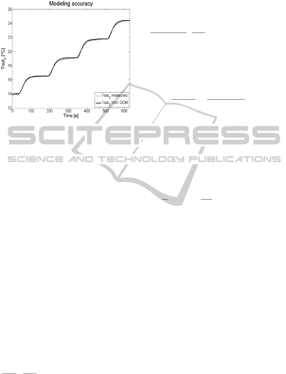
Figure 2: Accuracy of the OCM model for the chosen
operating point.
choice of the number of the discretization points
N+1 and on the values of the parameters α, β. For
the considered case, the values of N = 6, α = -0.06
and β = -0.53 were adjusted experimentally to ensure
the modelling accuracy comparable to the accuracy
of the FDM approximation. It can be noticed that the
order of the OCM approximation of the model (1) is
several times lower than the one for the FDM
approximation. Thus, in the case when the OCM
approximating model (7) is to be implemented
jointly with the controller (5), the computational
complexity of this approach is acceptable from the
practical viewpoint.
3.3 On-line Compensation for
Modelling Inaccuracies
Even if the parameters p
1
, p
2
, h
1
and h
2
are adjusted
based on the real measurement data collected from
the laboratory PHE to ensure relatively high
modelling accuracy of the OCM approximation (7),
in the practical cases it must be assumed that this
accuracy is limited and its compensation should be
included in the final form of the linearizing
controller. For this purpose, the idea suggested in
(Czeczot, 2003) for the adaptive control of the
distributed parameter biochemical reactors is
applied. Eq. (3) is completed with the single
additional time-varying parameter R
Y
that represents
the additive modelling inaccuracies:
)()()(
)()(
20,2
2
2
tRtYtuhtA
p
tF
dt
tdY
Y
.
(8)
Its value must be estimated on-line based on the
measurement data from the real process. After
discretization of Eq. (8) with the sampling time T
S
and defining the auxiliary variable w:
)(
)()(
)(
)(
)(
20,2
2
2
tR
tYtuhtA
p
tF
T
TtYtY
Y
tw
S
S
(9)
the scalar form of the Weighted Recursive Least-
Squares (WRLS) method can be applied to calculate
the estimate
Y
R
ˆ
:
)T(
)T(
1
)T(
)(
S
SS
tP
tPtP
tP
ff
,
(10a)
SS
T
ˆ
T
ˆˆ
tRtwtPtRtR
YYY
,
(10b)
where α
f
(0,1) is the forgetting factor.
After substituting the unknown parameter R
Y
by
its on-line estimate
Y
R
ˆ
and combining Eqs. (4) and
(8), the final discrete form of the linearizing
controller with the on-line compensation for the
modelling inaccuracies can be derived:
tRtYhtA
p
tF
tYY
h
tu
sp
ˆ
)(
)(
1
)T(
20,2
2
2
2
S
(11)
It should be implemented jointly with the on-line
numerical integration of the OCM approximation of
PHE (7) and computing of the estimation procedure
(9)-(10).
This approach is very similar to the Balance-
Based Adaptive Controller (B-BAC) suggested by
Czeczot (2001) for control of the nonlinear lumped
parameter systems and from this viewpoint, it can be
considered as the extension of the B-BAC
methodology for the control of the distributed
parameter heat exchangers. The major difference is
the direct application of the distributed parameter
model for the synthesis of the final form of the
control law.
4 SIMULATION RESULTS
This section shows the results of the simulation
experiments carried out to validate the control
performance of the suggested B-BAController (11).
The model (1) numerically integrated by FDM was
considered as the real system.
In the practice, the variations of the manipulated
variable u(t) = T
in1
(t) = T
1
(z=0,t) must be applied as
SimulationValidationoftheModel-basedControlofthePlateHeatExchangerwithOn-lineCompensationforModelling
Inaccuracies
661
the set point for the heating system with the inner
control loop that ensures possibly high tracking
properties. Thus, this actuating system has its own
dynamics that can deteriorate the performance of the
suggested PHE control system. During simulation
experiments, this dynamics was simulated by the
additional first-order lag system with unitary gain
and time constant adjusted as T
H
= 6 [s]. Readers
should note that this dynamics is not included in the
model applied for the synthesis of the
B-BAController (11) and it can be considered as the
unknown substitute dynamics of the actuating
system.
It was also decided to make the simulation
results more realistic by adding the additive random
noise to the measurement data from the controlled
temperature T
out2
and for the measured disturbances
F
1
, F
2
and T
in2
. This noisy data was used for
computing the estimation procedure (9) - (10) and
the manipulated variable by the control law (11).
The same data was also applied to excite the OCM
model used for approximation of the space
derivative
tA
z
tY
z 0,20
)(
for both the
estimation and the B-BAController.
The control performance of the suggested
B-BAController (11) is compared with the
performance of the conventional PI controller that is
still in use in the vast majority of the industrial
control loops. The PI controller was tuned based on
the process step response. Then, its tunings were
recalculated into the tunings of the B-BAController
(11) (namely, into its gain
and the forgetting factor
for the estimation procedure α
f
) by the tuning
method suggested by Stebel et al. (2014). Finally,
both controllers were retuned manually to ensure
possibly the same aperiodic tracking properties.
Thus, it can be assumed that both controllers were
tuned equivalently with the tunings k
r
= 1.7,
T
I
= 19.8 [s] for the conventional PI controller and
= 0.12, α
f
= 0.9949 for the B-BAController (11).
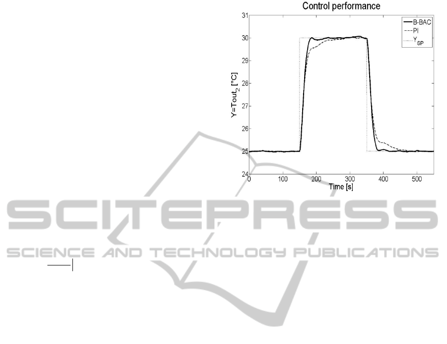
This equivalence can be seen in Fig. 3 that shows the
tracking properties of both controllers in the
presence of the indicated step changes of the set
point Y
sp
.
For this equivalent tuning, the disturbances
rejection for both controllers was investigated. The
system with the B-BAController (11) provides the
feedforward action from the measurable
disturbances F
2
and T
in2
, which results from the
direct application of the distributed parameter model
of PHE for the synthesis of the control law. Thus,
the significantly better disturbances rejection can be
obtained for the B-BAController (11), in the
Figure 3: Tracking properties of the considered
controllers. Noisy case.
comparison with the equivalently tuned conventional
PI controller.
The control performance of both controllers can
be seen in Figs. 4 - 6, at the presence of the step
changes of the respective disturbing signals F
2
, T
in2
and F
1
applied to the system. Upper diagrams of
each figure show the variations of the controlled
variable Y = T
out2
, while the lower diagrams show
the accuracy of the approximation of the space
derivative A
2,0
at the outlet of the cold water and
required for computing the estimation procedure (9)-
(10) and the control law (11). The FDM model is
used to compute the real value of A
2,0
while its
approximation is computed from the OCM model.
Readers should note relatively high accuracy of the
space derivative approximation and the fact that
such comparison is possible only in simulation - in
the practice, the real value of A
2,0
is always
unknown.
Note that at each case, the B-BAController (11)
ensures significantly shorter settling time with
smaller overregulation, even in the presence of the
changes of the disturbing flow rate F
1
, whose
measurement data is not included in the
B-BAController (11). At the same time, the presence
of the measurement noise does not corrupt the
control performance of the B-BAController (11)
more significantly as it does in the case of the
conventional PI controller, which makes the
suggested approach an promising alternative in the
industrial practical systems for the control of PHE.
SIMULTECH2014-4thInternationalConferenceonSimulationandModelingMethodologies,Technologiesand
Applications
662
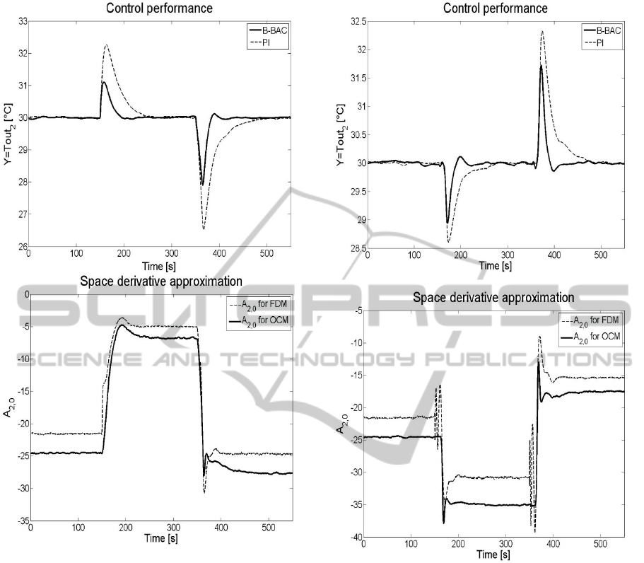
Figure 4: Rejection of the disturbing changes of the flow
rate F
2
: at t = 100 the step change of F
2
: 2.5 → 3.5;
at t = 300 the step change of F
2
: 3.5 → 1.5. Noisy case.
Upper diagram - controlled variable, lower diagram -
approximation of the space derivative A
2,0
.
5 CONCLUSIONS
This paper shows the potential possibility of the
application of the distributed parameter PHE model
for the synthesis of the model-based linearizing
controller. This approach is based on the low-degree
OMC approximation of the partial differential
equations describing the process dynamics. Based on
this approximation, the space derivative of the
controlled outlet temperature of the cold water is
computed and this derivative is directly included in
the control law to provide the feedforward action
and to compensate for process dynamics. The
Figure 5: Rejection of the disturbing changes of the inlet
temperature of the cold water T
in2
: at t = 100 the step
change of T
in2
: 15 → 20; at t = 300 the step change of
T
in2
: 20 → 10. Noisy case. Upper diagram - controlled
variable, lower diagram - approximation of the space
derivative A
2,0
.
potential modelling inaccuracies that would result in
the regulation offset are compensated by the
application of the on-line estimation of a single
additive parameter. The estimation procedure
requires the same measurement data and the same
OMC approximating model that are incorporated in
the suggested distributed parameter B-BAController.
The simulation experiments carried out under the
realistic scenarios considering the not modelled
dynamics of the actuating heating system show the
superiority of the suggested controller over the
conventional PI controller. The practical
applicability of these results is additionally
SimulationValidationoftheModel-basedControlofthePlateHeatExchangerwithOn-lineCompensationforModelling
Inaccuracies
663
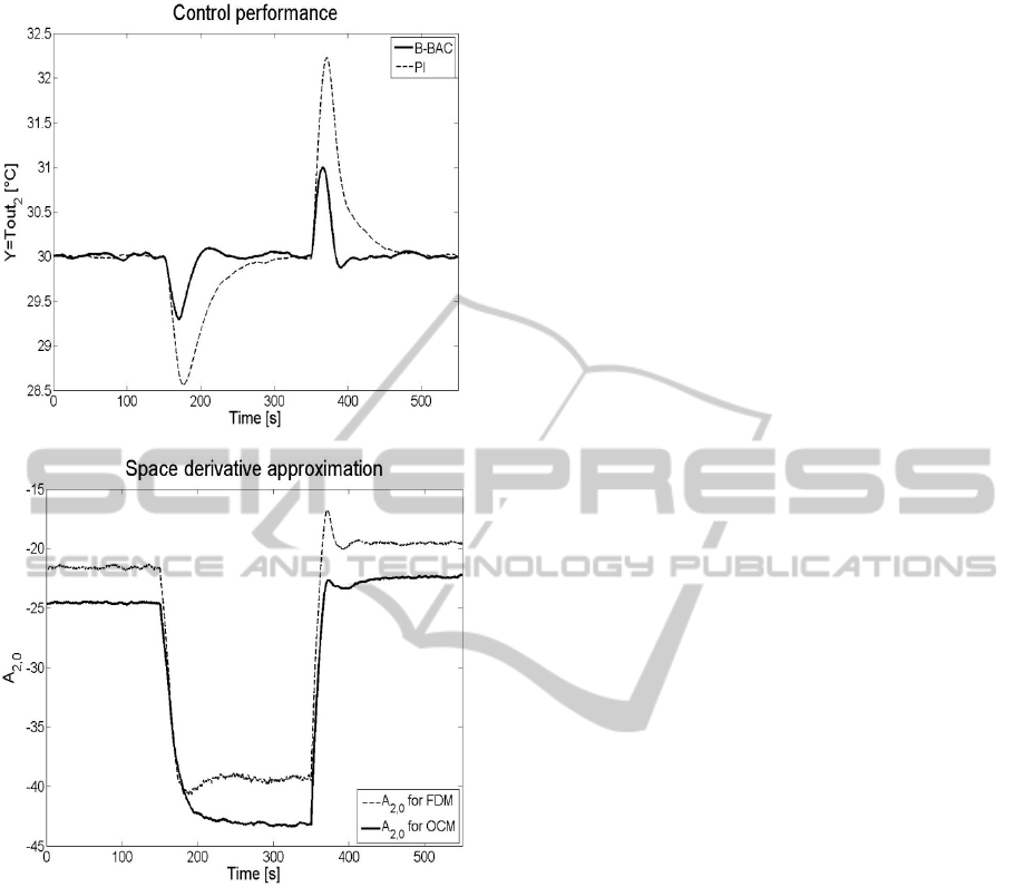
Figure 6: Rejection of the disturbing changes of the flow
rate F
1
: at t = 100 the step change of F
1
: 2.5 → 3.5;
at t = 300 the step change of F
1
: 3.5 → 1.5. Noisy case.
Upper diagram - controlled variable, lower diagram -
approximation of the space derivative A
2,0
.
supported by the fact that both the FDM model and
its OCM approximation were tuned and verified
based on the real measurement data collected from
the PHE operating in the laboratory heat exchange
and distribution setup.
From the practical point of view, the most
important advantage of the suggested
distributed parameter B-BAController is its
relatively low computational complexity and easy
tuning, which are combined with very good
disturbances rejection and resistance to the
measurement noise. Due to its low dimension, the
approximating OCM model can be easily integrated
numerically even in the programmable logic
controllers that already work in the existing
industrial control loops. Readers should note that
even if the computational power of the modern
PLCs is relatively high and still growing, the
practical implementations are still based on the
previous well established versions of the PLCs and
in the cases when a huge number of control loops
are to be operated simultaneously, their
computational power still can be a significant
limitation.
At the same time, the OCM model accuracy
ensures that there is no need to apply any state
observer technique for on-line approximation of the
space derivative of the controlled variable, which
significantly simplifies the tuning of the control
system. Surely, it is possible to use the suggested
OCM model for the synthesis of any well
established observer (Luenberger one or Kallman
filter) because this model is always observable but in
the considered case, this approach is not relevant. It
would require additional tuning of the observer,
which can be far from being trivial, especially if the
observer is to be nonlinear.
ACKNOWLEDGEMENTS
This work was supported by the Ministry of Science
and Higher Education under grants: BKM-UiUA
(Michal Fratczak, Pawel Nowak) and BK-UiUA
(Jacek Czeczot).
REFERENCES
Bastin, G., Dochain, D., 1990. On-line estimation and
adaptive control of bioreactors. Elsevier Science
Publishers B.V.
Bauer, M., Craig, I.K., 2008. Economic Assessment of
Advanced Process Control – a survey and framework.
Journal of Process Control, 18, 2–18.
Carver, M.B., Hinds, H.W., 1978. The method of lines and
advective equation. Simulation, 31, 59 – 69.
Czeczot, J., 2001. Balance-Based Adaptive Control of the
Heat Exchange Process. Proc. of 7
th
IEEE
International Conference on Methods and Models in
Automation and Robotics MMAR, Międzyzdroje,
853-858.
Czeczot, J., 2003. General methodology for the adaptive
control of a class of distributed parameter reactors.
Proc. of 9
th
IEEE Int. Conference on Methods and
Models in Automation and Robotics MMAR 2003,
Międzyzdroje, Poland.
Georgiadis M.C., Macchietto S., 2000. Dynamic
modelling and simulation of plate heat exchangers
SIMULTECH2014-4thInternationalConferenceonSimulationandModelingMethodologies,Technologiesand
Applications
664

under milk fouling. Chemical Engineering Science,
55, 1605-1619.
Gut J.A.W., Pinto J.M., 2003. Modeling of plate heat
exchangers with generalized configuration. Int.
Journal of Heat and Mass Transfer, 46, 2571-2585.
Henson, M.A., Seborg, D.E., 1997. Nonlinear Process
Control. Prentice Hall PTR.
Isidori, A., 1989. Nonlinear Control Systems: An
Introduction. 2
nd
edition. Springer Verlag.
Lagarias, J.C., Reeds, J.A., Wright, M.H., and Wright,
P.E., 1998. Convergence Properties of the Nelder-
Mead Simplex Method in Low Dimensions. SIAM
Journal of Optimization, 9(1), 112-147.
Maidi, A., Diaf, M., Corriou, J.P., 2009. Boundary
geometric control of a counter-current heat exchanger.
Journal of Process Control, 19, 297-313.
Maidi, A., Diaf, M., Corriou, J.P., 2010. Boundary control
of a parallel-flow heat exchanger by input-output
linearization. Journal of Process Control, 20, 1161-
1174.
Nelder, J.A., Mead, R., 1965. A simplex method for
function minimization. Computer Journal 7, 308 -
313.
Stebel, K., Czeczot, J., Laszczyk, P., 2014. General tuning
procedure for the nonlinear balance-based adaptive
controller. International Journal of Control, 87(1), 76-
89.
Villadsen, J.V., Michelsen, M.L., 1978. Solution of
differential equation models by polynomial
approximation. Prentice Hall, Englewood Cliffs, NJ.
SimulationValidationoftheModel-basedControlofthePlateHeatExchangerwithOn-lineCompensationforModelling
Inaccuracies
665
