Depth Sensor Placement for Human Robot Cooperation

Max St¨ahr, Andrew M. Wallace and Neil Robertson

School of Engineering and Physical Sciences, Heriot Watt University, Edinburgh, U.K.

Keywords:

Mobile Robot Sensor Placement, Collision Avoidance, Human Robot Cooperation.

Abstract:

Continuous sensing of the environment from a mobile robot perspective can prevent harmful collisions be-

tween human and mobile service robots. However, the overall collision avoidance performance depends

strongly on the optimal placement of multiple depth sensors on the mobile robot and maintains ﬂexibility

of the working area. In this paper, we present a novel approach to optimal sensor placement based on the

visibility of the human in the robot environment combined with a quantiﬁed risk of collision. Human visi-

bility is determined by ray tracing from all possible camera positions on the robot surface, quantifying safety

based on the speed and direction of the robot throughout a pre-determined task. A cost function based on

discrete cells is formulated and solved numerically for two scenarios of increasing complexity, using a CUDA

implementation to reduce computation time.

1 INTRODUCTION

Mobile service robots have signiﬁcant potential for

factory automation, however safety is of paramount

importance. The main concern in human robot co-

operation is sudden, unforeseen contact between a

robot and a human and of severe force and pres-

sures on the human body. Approaches to safe hu-

man robot cooperation can be divided into two cat-

egories: limiting the consequences of an impact and

avoiding a collision. In the former case, the in-

juries of unexpected human-robotimpacts can be lim-

ited by lightweight/compliant mechanical design of

the manipulator and post-collision reaction strategies

(De Luca et al., 2006).

However, reducing risk by mechanical design also

reduces the payload of the robot system, and safety

may well be compromised in unstructured environ-

ments. In the latter case, collision avoidance based on

exteroceptive sensors is independent of the payload

and mass of the robot (Angerer et al., 2012). Early

developments utilized ﬁxed, mounted intensity cam-

eras (Ebert and Henrich, 2002) (Henrich and Gecks,

2008) to detect overlapping silhouettes of robots and

obstacles. Later developments used 3D environment

perception in real time to improve collision avoidance

for human robot cooperation and Euclidean distance

related robot velocity controls (Fischer and Henrich,

2009) (Graf et al., 2010) (Lenz, 2012). However,

surveillance of the operational area of a mobile robot

by a static sensor network is undesirable because

many sensors are required to cover a large area, and

it lacks ﬂexibility if the task or operating environment

is changed. Rather, mounting the sensors on the robot

so that they have a dynamic perspective gives much

greater ﬂexibility.

The major drawback of this approach is the prob-

able interaction between the robot-mounted sensors

and the mobile platform and manipulators which can

result in large shadowed volumes and consequent un-

seen collisions. A necessary strategy is to raise the

number of sensors to decrease shadowed volumes, but

computational and power resources are limited. The

problem of optimal placement becomes even more

challenging as the sensor positions change with robot

movement.

1.1 Related Work

We pose the problem as one of optimization with re-

spect to a cost function that maximises the visibility

with regard to regions of potential robot human col-

lision. Systematic optimization of static camera se-

tups is a known challenge in surveillance tasks, aim-

ing to minimize the demanded resources while con-

currently maximizing surveillance. The visibility as-

pect of the problem can be regarded as an extension

of the art gallery problem which consists of ﬁnding

the minimum number of cameras to survey a given

space (O’rourke,1987). The distinction from the orig-

311

Stähr M., M. Wallace A. and M. Robertson N..

Depth Sensor Placement for Human Robot Cooperation.

DOI: 10.5220/0005017103110318

In Proceedings of the 11th International Conference on Informatics in Control, Automation and Robotics (ICINCO-2014), pages 311-318

ISBN: 978-989-758-040-6

 2014 SCITEPRESS (Science and Technology Publications, Lda.)

inal art gallery problem is that our guard is moving

along on a pre-deﬁned robot path and our objective is

to maximise visibility of regions where the possibility

of collision is greatest.

Numerical solutions decompose the workspace

into equal sized cells and assign to each a binary at-

tribute indicating whether or not it is seen by a sensor

at a certain position. The number of sensors is raised

and their positions are varied until the optimum is

found (Dhillon et al., 2002). Often the system perfor-

mance has been described as the detection of certain

features in the surveyed scene such as humans (Yao

et al., 2008), (Bodor et al., 2007) or robot paths (Niko-

laidis et al., 2009) which are not equally distributed

over the grid. A cost function is utilized to factor the

quality of feature recognition at a certain cell from a

known sensor position. Including the presence of oc-

cluders, e.g. other humans (Mittal and Davis, 2008)

or pillars (Chen and Davis, 2008) improves the over-

all performance of such systems in dynamic surround-

ings.

The grid is extended to a voxel grid for a three

dimensional feature distribution. In the work of

Flacco (Flacco and De Luca, 2010) the position of

depth and presence sensors is optimized for a ﬁxed

robot arm and human sharing the same workspace. A

probabilistic visibility approach for pre-deﬁned robot

motion and human presence distribution is delineated.

Sensor mounting positions are restricted to the sur-

rounding wall and obstructions include the robot arm

and the human itself as well as static environment ob-

jects such as walls and tables. We extend the approach

of Flacco to dynamic environments with pre-deﬁned

human and robot movements. The major extensions

to Flacco’s work presented here are the use of moving

cameras on the mobile robot and the introduction of

a safety criterion which reﬂects the consequences of

human robot collisions.

Concepts of robot safety were developed mainly

in human aware robot motion planners. The human

position is determined and the robot’s velocity or tra-

jectory is adapted according to the distance (Had-

dadin, 2013), robot arms inertia (Kulic and Croft,

2007) and direction (Sisbot et al., 2010). More com-

plex approaches build up velocity related scalar ﬁelds

for each robot arm link and superimpose them on a

resulting ﬁeld according to the current joint conﬁg-

uration and speed (Lacevic and Rocco, 2010). The

number of sample points is bounded to fulﬁl real time

constraints of the motion controllers. Here, we extend

the scalar ﬁeld of Lacevic to the robot mesh and apply

it to arbitrary and complex robot shapes and geomet-

ric structures because the source of danger is not the

geometric centre of link, rather the solid outer shape

of the robot.

We have chosen to formulate a numeric approach

for optimal depth sensor placement for collision

avoidance on mobile robots. The working area is de-

composed into cells of equal size and each cell is as-

signed with both binary visibility and scalar danger

attributes representing the potential collision in this

cell. We specify the vertices of a mesh of the outer

robot shape as potential sensor positions and sample

all three rotational degrees of freedom for each posi-

tion. A cost function depending on the sensor’s po-

sition and orientation is introduced and numerically

minimized by complete enumeration as this is an of-

ﬂine process.

This paper is organized as follows. Sections 2

and 3 describe the robot, human and sensor model as

well as the work cell decomposition based on visibil-

ity. Section 4 introduces the quantifying safety mea-

surement utilized in the cost function introduced in

section 5. Section 6 provides two experiments with

increasing complexity and section 7 summarises the

results and gives an outlook on future work.

2 ROBOT AND HUMAN

MODELING

We model the robot as an articulated, rigid body chain

consisting of static meshes and time variant homoge-

neous transformations T

at time t. The position and

orientation of the m-th link w. r. t. a global coordinate

origin can be expressed by:

...

m−1

(1)

in which

i−1

describes the homogenous link-to-link

transformation following the Denavit-Hartenberg-

convention and mapping a robot state vector q

r,t

= [x

r,t

1,t

···a

6,t

]

(2)

in which x

r,t

, y

r,t

, θ

r,t

expresses the translational and

rotational displacement of the mobile platform associ-

ated with the mobile robot frame T

mr,t

and a

1,t

···a

6,t

are the joint angles of the 6R (6 rotatory joints) robot

arm at time t. The complete robot shape RM

is de-

ﬁned as the union of all meshes M

transformed ac-

cording to their parent link frame T

n,t

at time t.

The human is represented as a rigid stick ﬁg-

ure considering Cartesian position and gaze direction.

Following that simpliﬁcation the human state vector

h,t

at time t is expressed as:

h,t

= [x

h,t

]

(3)

and associated with the frame T

h,t

having an equiva-

lent state vector to the mobile platform.

ICINCO2014-11thInternationalConferenceonInformaticsinControl,AutomationandRobotics

312

3 SENSOR MODELING

Each of the depth sensors is modelled as a virtual

camera. Each ray that passes through the focal cen-

tre F

assigns its data to a point on the image plane

IP. The image coordinates x on IP are expressed by

the pin hole projection equation:

x = PX = KEX (4)

The intrinsic parameters are stored in the camera ma-

trix K, and the extrinsic homogenous transformation

E is used to obtain the projection matrix P. All Carte-

sian points X on the same ray lead to the same value

of x. The depth of a Cartesian point to a known cam-

era position is given by:

depth(X) = kF

− Xk (5)

We store the depth information along the ray of the

corresponding pixel on the IP and name it depending

on its source.

3.1 Sensor Position

As we mount the sensor on the mobile robot the posi-

tion and orientation of the sensor depends at least on

the frame T

mr,t

, thus our objective is to optimize the

sensor position vector q

w.r.t to T

mr,t

= [x y z roll pitch yaw]

(6)

In this work we make a simpliﬁcation and attach the

focal centre of the camera to one point of the complete

initial robot mesh RM

for a

...a

= 0. On a real

robot the focal centre cannot be attached directly to

the robot hull as there are mounting constraints, such

as minimum distance to the hull or forbidden regions

such as drives, gripper, wheels or laser scanners. In

this work we deﬁne the set of all possible camera po-

sition on the robot as:

= {q

∈ R

c,1

... q

c,3

∈ RM

∧

− π < q

c,4

...q

c,6

≤ π}

(7)

As the camera may be attached to the robot

arm, its position and orientation may vary for any

...a

6= 0. We compute the resulting position and

orientation of the sensor by determining the local,

time invariant transformation

between the cam-

era frame T

in the base of the link frame T

to which

it is attached, building the closed kinematic chain via

−1

∀ q

...a

= 0) (8)

Now we can extend the kinematic chain from equa-

tion 1 by the time invariant transformation

to:

...

m−1

∀ q

(9)

and determine the camera frame w.r.t to the mobile

platform

for all q

r,t

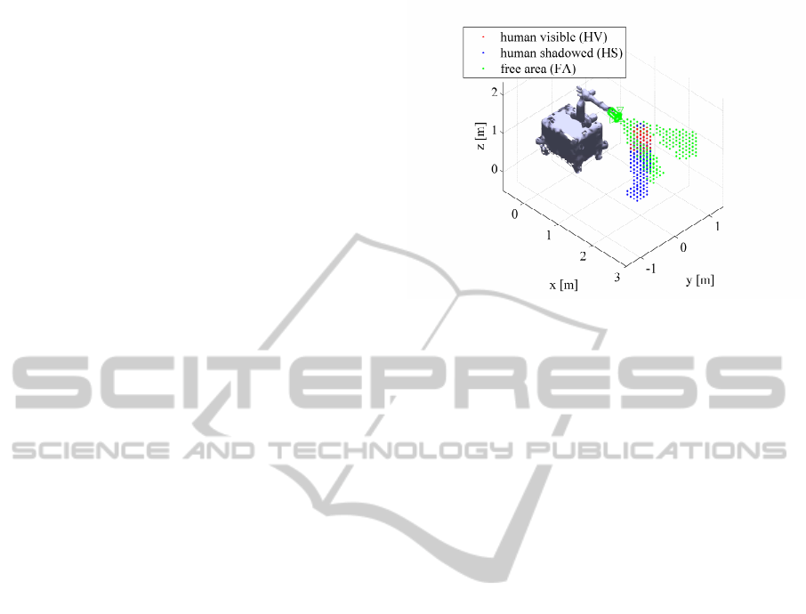
Figure 1: workspace decomposition.

3.2 Work Cell Decomposition

We decompose the mobile platform centered cell WC

around a mobile robot in N regular cells of equal edge

length. Each cell belongs to one of the following set.

The free area FA represents the set of all Cartesian

cells which are in the ﬁeld of view (FOV) of the depth

sensor but do not belong to either the robot R, the en-

vironment E (static objects) or the human H. The

dark area DA sums all the cells outside the FOV for

which we have no information. In contrast to pre-

vious work Flacco (Flacco and De Luca, 2010) we

do not distinguish between sources of DA, rather we

maximise the visible human cells HV, which are the

difference set of human H and human shadowed HS

sets. Summarizing, at any time t, the following rela-

tion holds:

WC(t) = FA(t) ∪ DA(t) ∪ R(t) ∪ E(t) ∪ H(t)

H(t) = HV(t) ∪ HS(t)

HS(t) = H(t) \ HV(t)

(10)

Following the notation of a depth sensor from

equation 5, we deﬁne two depth images: the envi-

ronment depth map E

and the human depth map

. For a pixel x associated with Cartesian points

lying on the ray PX = x that intercept the robot or the

environment, we set

(x) = min

X∈R∪E

PX=x

depth(X) (11)

and

(x) = min

X∈H

PX=x

depth(X) (12)

if it intercepts the human body. As we ray trace the

environment and the human separately we can now

compare the depth image pixel by pixel to determine

DepthSensorPlacementforHumanRobotCooperation

313

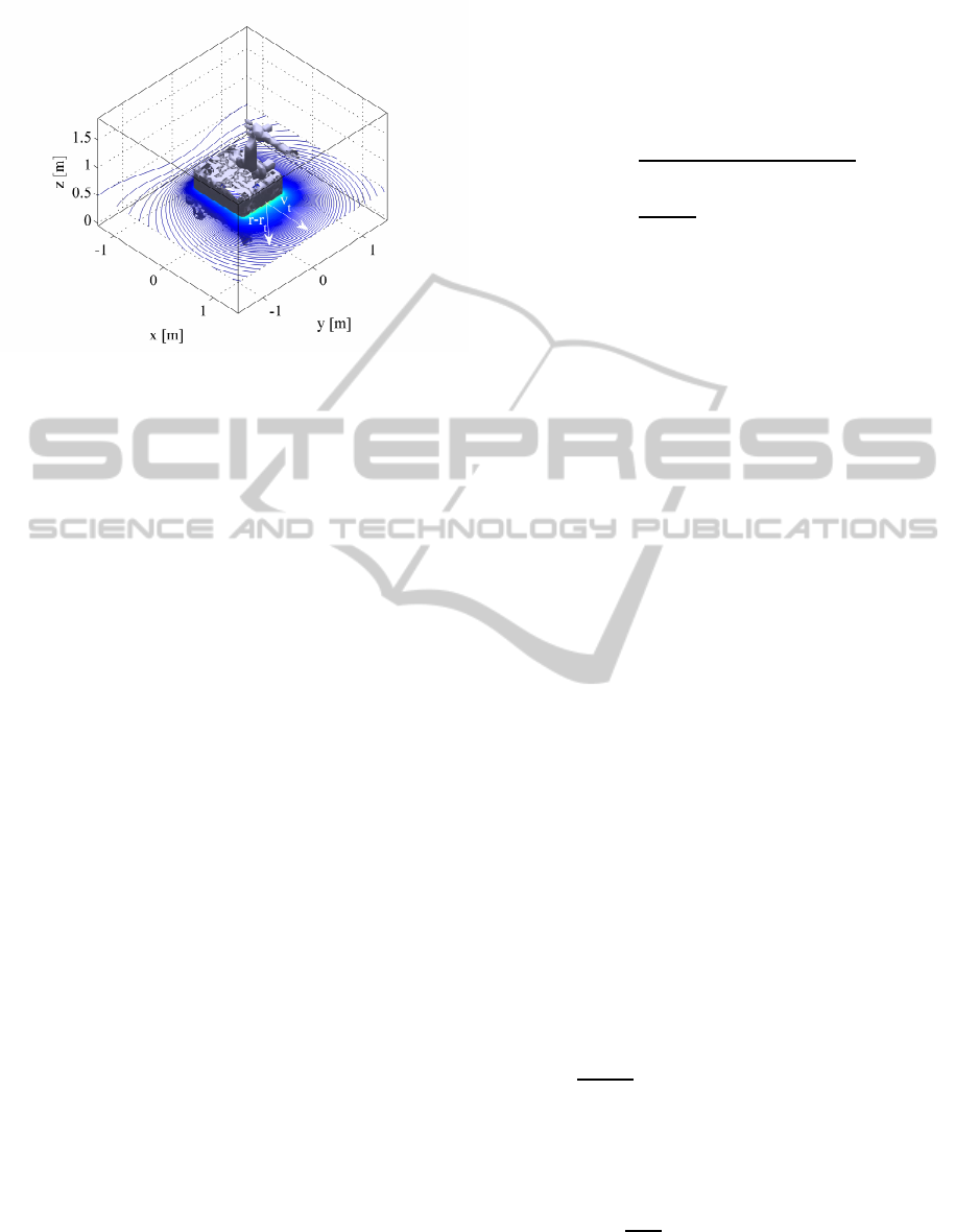
Figure 2: kinetostatic danger ﬁeld applied to mobile robot

at z=0.5m for ˙q

r,t

= [1.0,0. . . 0]

the human shadowed volume and free area as follows:

FA = {X ∈ WC :d

min

≤ depth(X) < d

max

AND

(PX) > depth(X) AND

(PX) > depth(X)}

(13)

HV = { X ∈ H :d

min

≤ depth(X) < d

max

AND

(PX) ≤ depth(X) AND

(PX) < E

(PX)}

(14)

for all Cartesian points. As our goal is to optimize for

multiple sensors we deﬁne a sensor state vector s for

n sensors as the n-times product set of P

s ∈ (P

)

(15)

representing position and orientation of the nth sensor

following the deﬁnition of P

in equation 7. The re-

sulting free and human shadowed areas for n sensors

can be described respectively as the union intersec-

tions of the corresponding sets for each single cam-

era:

c=1...n

(16)

[

c=1...n

(17)

4 SAFETY COSTS

In this work a kinetic-static danger ﬁeld (KSDF) cap-

tures the complete state for safe motion planning of

an articulated robot (Lacevic and Rocco, 2010) to

quantify safety. Two scalar distance related ﬁelds: a

quadratic decreasing dynamic ﬁeld and a linear de-

creasing static ﬁeld, are superimposed. The dynamic

ﬁeld does not just consider the distance between the

source of danger r

and sample point r, it also includes

the angle between the translational velocity vector ~v

and the direction vector r − r

as expressed in equa-

tion 18 and illustrated in ﬁgure 2.

DF(r,r

,~v

) =

|~v

|[γ+ cos∠(r− r

,~v

)]

|r− r

(18)

The constant γ ≥ 1 eliminates the change of sign at-

tribute of the cosine. The original ﬁeld of application

of the KSDF is human aware robot motion planning,

thus the number of points r on the robot are limited to

discrete points on the link of the robot arm between

two joints. This approach has been extended to all

points of an arbitrary complexrobot mesh RM

at time

t as the source of danger is not the geometric link but

the solid outer hull of the robot. The meshes have

been re-sampled at a unique resolution of 5 cm so the

danger ﬁeld is equally distributed over the robot. The

velocity vector v

is calculated using forward kinemat-

ics from equation 1 and the Jacobian of each transfor-

mation

i−1

The danger ﬁeld is accumulated over all vertices

of the robot mesh RM

for each centre of cell C

formulated in equation 19. The resulting scalar ﬁeld

is illustrated in ﬁgure 2 for a height of z = 0.5 m and a

translational velocity of 1 m/s in the positive x direc-

tion.

KSDF(C

) =

|RM

∑

j=0

DF(C

,RM

( j), v

(RM

( j))) (19)

5 OPTIMAL DEPTH SENSOR

PLACEMENT

Using the components deﬁned in the previous sec-

tion, we can compute a cost function with additional

assigned weights, w

and w

to compute a single

scalar value for a given camera state vector s.

J(s) =

∑

j=1

∑

i=1

s, j

)KSDF(C

)−

s, j

)KSDF(C

)

(20)

for

∑

i=1

KSDF(C

)

The cost function J(s) sums all the human shadowed

cells multiplied by the corresponding KSDF value.

ICINCO2014-11thInternationalConferenceonInformaticsinControl,AutomationandRobotics

314

Positions, in which the human is close to the robot

path and not seen are prioritised. The cost function is

lowered by the weighted cells of FA to maximize the

visible area for equal human visibility. w

is much

larger than w

so that maximizing the free area is a

secondary objective.

The algorithm for optimal depth sensor placement

is divided into two phases: initiation and optimiza-

tion. During the initialization phase the human shad-

owed volume and the free area for each possible ge-

ometric arrangement are determined as illustrated in

algorithm 1. A geometric arrangement is deﬁned as

a combination of q

, q

r,t

and q

h,t

. We specify the set

as the set of all possible q

with an equivalent P

for robot positions and P

for human positions. For

each member of P

we determine HS and FA for all

members of P

= P

× P

. If for at least one member

of P

the relation H 6= HS holds, then q

is stored in

the set of valid camera position P

valid

, thus the human

is visible in at least one geometric arrangement of P

To reduce computation in the optimization phase, we

neglect all q

which have no contribution to the cost

function (1).

In the optimization step (see algorithm 2) we de-

ﬁne S as the set of all possible camera state vectors s

for a given set, P

valid

, and a number of cameras n

S = {s ∈ P

valid

: no repetition of s} (21)

In this work we used a single camera type and the

order of q

in vector s does not matter because each

sensor has equal visibility for the same q

. Conse-

quently, the cardinality of S can been described by the

binomial coefﬁcient:

|S| =



valid



(22)

During optimization we raise the number of cameras

until complete human visibility is reached. We are

looking for the minimum cost in which the human is

completely visible which is expressed as |HS

| = 0 for

all positions in P

The optimisation step implies that the human will

be visible for a ﬁnite number of cameras, however if

the human is covered behind a static obstacle (e.g. a

pillar) that is not the case. In the future we will in-

troduce a second criterion to check human visibility

compared to the least number of sensors. The opti-

misation will be stopped if an additional sensor does

not improve human visibility and the solution with the

lowest cost from the previous number of sensors will

be regarded as optimum.

Data: P

, P

Result: P

valid

foreach q

∈ P

qcvalid = false;

foreach q

r,t

∈ P

build

from q

r,t

;

adjust E according to

−1

;

adjust RM

according to q

r,t

;

assign RM

to R;

ﬁnd

from RM

and q

r,t

;

ray trace EDM for current

;

foreach q

h,t

∈ P

ﬁnd

;

adjust H according to

;

ray trace HDM for current

;

determine HS and FA;

add HS and FA to HStemp and

FAtemp;

if H 6= HS then

qcvalid = true;

end

if qcvalid then

add q

to P

valid

;

store HStemp and FAtemp;

end

Algorithm 1: Initialization step.

6 EXAMPLES OF OPTIMAL

PLACEMENTS

We have performed two experiments with increasing

complexity. Both experiments were performed with a

depth camera model of 64 × 50 pixel resolution and

◦

× 40

◦

FOV. The robot centred workspace had di-

mensions of 6 m in width and length and 3 m in

height. It was decomposed into 131.072 cells hav-

ing an equal edge length of 9.375cm. We used a fast

voxel traversal algorithm for ray tracing (Amanatides

and Woo, 1987) because our environment model con-

sists of an occupancy grid and we are not interested in

very accurate depth images, instead we focus on small

computational cost. All experiments were performed

on a workstation equipped with an Intel Xeon W3680

and 18GB of ram. The ray tracing and cost function

evaluation was performed using CUDA on a NVidia

GTX670 device with 1536 Cuda cores.

In the ﬁrst experiment we evaluated all possible

DepthSensorPlacementforHumanRobotCooperation

315

Data: P

valid

Result: s

opti

= 1;

mincosts = MAX;

while true do

S = (P

valid

)

;

abort = false;

foreach element s of S do

costs = J(s);

if |HS

| = 0 then

abort = true;

end

if costs < mincosts then

mincosts = costs;

opti

= s;

end

if abort then

break;

end

+ +;

end

Algorithm 2: Optimization step.

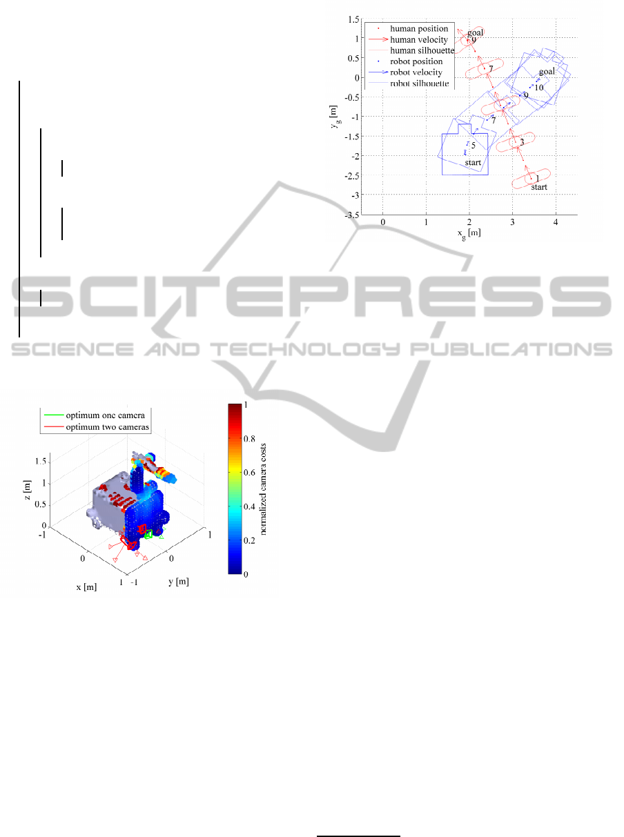
Figure 3: Results for multiple sensors, one human robot

position.

camera positions and orientation for a single robot hu-

man position pair. The second experiment evaluates

a path scenario displayed in ﬁgure 4 in which the hu-

man crosses the robot path. In the second scenario we

were just able to compute the cost function for a sin-

gle camera position because of limited computational

resources.

6.1 Multiple Sensors, one Human Robot

Position

The geometric arrangement of the ﬁrst experiment is

illustrated in ﬁgure 1. The human is standing at 2.5

Figure 4: Human and robot path.

m in the positive x direction in front of the robot.

We have evaluated 2,590 possible camera positions

on the robot and sampled each angular degree of free-

dom 10 times, thus the resulting number of samples

is 2,590,000. The minimum cost value for all an-

gles of the same Cartesian position of P

valid

is illus-

trated by the colour value of the Cartesian point in

ﬁgure 3. |P

valid

| was 241,660, thus the amount of

sample points for the multi camera optimisation was

reduced to 10.71 % of the original amount of position

and orientations. This reduction is important as the

number of samples to be evaluated for each camera

is increased according to the binomial coefﬁcient of

equation 22.

The complete human visibility was found with

two cameras after 176 sec, as displayed in ﬁgure 3.

The optimal solution for one camera is close to the

ground as the distance to the human body increases,

which results in a large volume covered. The sec-

ond camera for the optimal solution for two cameras

is almost overlapping with the optimal solution for a

single camera because the second camera maximizes

the secondary criterion, the visibility of free area.

6.2 One Sensor, Multiple Human Robot

Positions

In the second experiment we evaluated the camera

costs for a single camera in a dynamic scenario with

human and robot trajectories displayed in ﬁgure 4.

The robot trajectory was generated using the origi-

nal path planner from the robot manufacturer

giving

equivalent paths in real world. The human path was

generated using the motion planner for the holonomic

http://www.neobotix-robots.com/industrial-robot-mm-

800.html

ICINCO2014-11thInternationalConferenceonInformaticsinControl,AutomationandRobotics

316

Figure 5: Best, medium and worst camera position on the

robot.

0 1 2 3 4 5 6 7 8 9 10 11 12 13 14 15 16

robot positions of P

average costs for all elements of P

worst

average

best

Figure 6: Best, medium and worst camera position on the

robot.

mobile robots of Siegwart (Siegwart et al., 2011) tak-

ing the human motion constraints of Brogan (Brogan

and Johnson, 2003) into account. The paths were

sampled at a time step of 1 sec. The cardinality of

was 156 consisting of 9 human and 16 robot po-

u [px]

v [px]

10 20 30 40 50

human visibility per pixel

0.05

0.1

0.15

0.2

0.25

0.3

Figure 7: Human visibility per pixel for the best camera

position.

sitions from which 143 conﬁgurations were without

collisions and considered in the cost function. All

2,590,000 camera positions were evaluated in 366 sec

utilizing the cost function from equation 20 for multi-

ple human robot positions.

The worst, average and best camera positions for

the second scenario are illustrated in ﬁgure 5. The av-

erage costs over all human positions for a single robot

position are compared in ﬁgure 6. All three camera

positions have their minimum at p

r,1

and p

r,12

respec-

tively and their maximum at p

r,6

. The robot does not

move instantly, thus the robot translational speed is

zero followed by a clockwise turn. Consequently the

KSDF is almost zero at p

r,1

which causes very low

costs for all sensor positions. The maximum cost

value is reached at p

r,6

because the robot is almost in-

tersecting the human path, therefore the human robot

distance is very low which causes a very high KSDF

value for human shadowed cells. The second mini-

mum at p

r,12

is caused by a second stop before turning

counter clockwise which results in better performance

for the average position as it is now turned towards

the human path. All three camera positions perform

equally if the human is not seen by any of them be-

cause the free area behaves as a secondary criterion

as explained in section 5.

The human visibility at p

r,6

for all human posi-

tions of the best camera position can be seen in ﬁg-

ure 7. The best camera position covers the ﬁrst half of

the human path, nevertheless the human is just visible

in one third of the human positions. Multiple sensors

are required to increase human visibility and improve

collision avoidance.

7 CONCLUSION

A novel approach to the placement of multiple depth

sensors on a mobile robot for human robot cooper-

ation is presented in this work. We have quanti-

ﬁed the danger of collision between a human and a

robot in pre-determined task positions and combined

this with maximum human visibility to obtain a nu-

merically solvable cost function. Experiments have

shown promising results for optimal camera place-

ment using the cost function, but in future work these

need to be further evaluated by running more com-

plex scenarios in simulation before moving to real

world scenarios. Even simple scenarios with small

robot and human trajectories require 4.5 days for sin-

gle camera optimisation with poor human visibility.

However, real world cooperative human robot sce-

narios consist of numerous tasks, task execution or-

ders and varying robot and human trajectories. Even

DepthSensorPlacementforHumanRobotCooperation

317

though computation is ofﬂine, exhaustive enumera-

tion of a large number of potential robot, sensor and

human positions combined with ﬁnite computational

resources demands further research into both the can-

didate function for single and multi-camera place-

ment, and an optimisation strategy that does not re-

quire such exhaustive enumeration. Promising ap-

proaches are genetic algorithms (Dunn et al., 2006)

or simulated annealing (Mittal and Davis, 2008) for

highly non-linear optimisation to reduce the number

of camera state vectors s to be evaluated. Fast opti-

misation strategies enable online robot path planning

for full human visibility and best collision avoidance

performance.

ACKNOWLEDGEMENTS

The authors would like to acknowledge the support

of the University of Applied Sciences, Ingolstadt

and the Engineering and Physical Research Council

(EP/J015180/1 Sensor Signal Processing).

REFERENCES

Amanatides, J. and Woo, A. (1987). A fast voxel traversal

algorithm for ray tracing. In Proceedings of EURO-

GRAPHICS.

Angerer, S., Strassmair, C., Staehr, M., Roettenbacher, M.,

and Robertson, N. (2012). Give me a hand. In Tech-

nologies for Practical Robot Applications (TePRA),

2012 IEEE International Conference on.

Bodor, R., Drenner, A., Schrater, P., and Papanikolopoulos,

N. (2007). Optimal camera placement for automated

surveillance tasks. Journal of Intelligent & Robotic

Systems.

Brogan, D. C. and Johnson, N. L. (2003). Realistic hu-

man walking paths. In Computer Animation and So-

cial Agents, 2003. 16th International Conference on.

Chen, X. and Davis, J. (2008). An occlusion metric for se-

lecting robust camera conﬁgurations. Machine Vision

and Applications.

De Luca, A., Albu-Schaffer, A., Haddadin, S., and

Hirzinger, G. (2006). Collision detection and safe re-

action with the dlr-iii lightweight manipulator arm. In

Intelligent Robots and Systems, 2006 IEEE/RSJ Inter-

national Conference on. IEEE.

Dhillon, S. S., Chakrabarty, K., and Iyengar, S. S. (2002).

Sensor placement for grid coverage under imprecise

detections. Information Fusion, 2002. Proceedings of

the Fifth International Conference on.

Dunn, E., Olague, G., and Lutton, E. (2006). Parisian

camera placement for vision metrology: Evolutionary

Computer Vision and Image Understanding. Pattern

Recognition Letters.

Ebert, D. M. and Henrich, D. D. (2002). Safe human-robot-

cooperation: Image-based collision detection for in-

dustrial robots. In Intelligent Robots and Systems,

2002. IEEE/RSJ International Conference on. IEEE.

Fischer, M. and Henrich, D. (2009). 3D collision detec-

tion for industrial robots and unknown obstacles us-

ing multiple depth images. Advances in Robotics Re-

search.

Flacco, F. and De Luca, A. (2010). Multiple depth/presence

sensors: Integration and optimal placement for hu-

man/robot coexistence. In Robotics and Automa-

tion (ICRA), 2010 IEEE International Conference on.

IEEE.

Graf, J., Puls, S., and W¨orn, H. (2010). Recognition and un-

derstanding situations and activities with description

logics for safe human-robot cooperation. In COGNI-

TIVE 2010, The Second International Conference on

Advanced Cognitive Technologies and Applications.

Haddadin, S. (2013). Towards Safe Robots: Approaching

Asimov’s 1st Law. Springer Publishing Company, In-

corporated.

Henrich, D. and Gecks, T. (2008). Multi-camera collision

detection between known and unknown objects. In

Distributed Smart Cameras, 2008. ICDSC 2008. Sec-

ond ACM/IEEE International Conference on. IEEE.

Kulic, D. and Croft, E. (2007). Affective state estimation

for human–robot interaction. Robotics, IEEE Trans-

actions on.

Lacevic, B. and Rocco, P. (2010). Kinetostatic danger ﬁeld -

a novel safety assessment for human-robot interaction.

In Intelligent Robots and Systems (IROS), 2010.

Lenz, C. (2012). Fusing multiple kinects to survey shared

human-robot-workspaces. Technical report, Techni-

cal Report Technical Report TUM-I1214, Technische

Universit¨at M¨unchen, Munich, Germany.

Mittal, A. and Davis, L. (2008). A General Method for

Sensor Planning in Multi-Sensor Systems: Extension

to Random Occlusion. International journal of com-

puter vision, 76(1):31–52.

Nikolaidis, S., Ueda, R., Hayashi, A., and Arai, T. (2009).

Optimal camera placement considering mobile robot

trajectory. In Robotics and Biomimetics, 2008. IEEE

International Conference on. IEEE.

O’rourke, J. (1987). Art gallery theorems and algorithms,

volume 1092. Oxford University Press Oxford.

Siegwart, R., Nourbakhsh, I. R., and Scaramuzza, D.

(2011). Introduction to autonomous mobile robots.

MIT Press.

Sisbot, E., Marin-Urias, L., Broquere, X., Sidobre, D., and

Alami, R. (2010). Synthesizing robot motions adapted

to human presence. International Journal of Social

Robotics.

Yao, Y., Chen, C.-H., Abidi, B., Page, D., Koschan, A.,

and Abidi, M. (2008). Sensor planning for automated

and persistent object tracking with multiple cameras.

In Computer Vision and Pattern Recognition, 2008.

IEEE Conference on. IEEE.

ICINCO2014-11thInternationalConferenceonInformaticsinControl,AutomationandRobotics

318