
Manifold Embedding based Visualization of Signals
Hee Il Hahn
Department of Information and Communications Eng., Hankuk University of Foreign Studies, 89 Wangsan, Mohyun,
Yongin , Kyonggi-Do, 449-791, Korea
Keywords: Manifold Embedding, Commute Time, Patch Graph, Graph Laplacian.
Abstract: We address the problem of transforming statistically stationary waveform signals into their intrinsic
geometries by embedding them into two or three dimensional space for the purpose of visualizing them. The
graph Laplacian based manifold embedding algorithms basically generate geometries intrinsic to the signal
characteristics under the conditions that it is smooth enough and sufficient number of patches are extracted
from it. Especially, commute time is known to have the properties of shrinking the mutual distance between
two points as the number of paths connecting them increases, which makes it possible to align the
statistically different patches in the form of curves. Extensive experiment is conducted with speeches and
musical instrumental sounds to investigate the relevance of the waveforms to their own inherent geometries.
1 INTRODUCTION
If data lies in a higher dimensional space, it is very
hard to imagine what it looks like. However, if it is
possible to visualize it in a two or three dimensional
space, it can be a meaningful clue for a desired
output in the area of pattern recognition or machine
learning. When data set lies on or close to a linear
subspace, PCA(principal component analysis) is
most useful and optimal for dimensionality
reduction in terms of maintaining maximum
variance of the data set. However, when data set lies
on a nonlinear space, PCA introduces severe error.
The manifold learning algorithms replace PCA on a
nonlinear space.
Over last decades, there have been several
different embedding algorithms developed for
dimensionality reduction in manifold ways. Isomap
(Tenenbaum et al, 2000) and locally linear
embedding (Roweis and Saul, 2000) are known to be
the first manifold learning algorithms. Laplacian
eigenmap (Belkin and Niyogi, 2003), based on ideas
from spectral graph theory, attempts to represent
data points using information involved in the
eigenvalues and eigenvectors of the graph Laplacian.
The spectral graph theory analyzes how information
diffuses with time across the edges connecting nodes
via eigenvalues and eigenvectors of the Laplacian
matrix of the graph. The general principle of
computing an eigenspace is to reduce the complexity
of a problem by focusing on a few relevant
quantities and dismissing others. Many authors
recently began to consider random-walk based
similarity measure on the graph. The hitting time
,hij of a random walk on a graph is defined as
the expected time for a random walk on a graph to
start from a node
i
v to arrive at a node
j
v .
However, it may not be symmetric, that is
,,hij h ji , which makes it inappropriate for a
distance measure between pairs of nodes. An
alternative measure for the hitting time is a commute
time
,cij , which is defined as the average time
taken for the random walk to travel from node
i
v to
reach
j
v for the first time and then return to
i
v , i.e.,
,,,cij hij h ji. Commute time provides a
distance measure between any pair of vertices. (Qiu
and Hancock, 2007) showed the commute time can
be computed from the Laplacian spectrum using the
discrete Green’s function. (Taylor, 2011) proposed
methods to organize the patches extracted from
images or waveform signals according to the graph-
based metrics. They showed the embedding of the
set of patches based on the eigenfunctions of the
graph Laplacian can concentrate even the patches
including high frequency components. Their recent
studies on the patch graph and its embedding give
convincing ideas of analyzing signals from the
184
Hahn H..
Manifold Embedding based Visualization of Signals.
DOI: 10.5220/0005017801840189
In Proceedings of the 11th International Conference on Informatics in Control, Automation and Robotics (ICINCO-2014), pages 184-189
ISBN: 978-989-758-039-0
Copyright
c
2014 SCITEPRESS (Science and Technology Publications, Lda.)

geometrical point of view. Although the usual
shortest path distance is most common metric on a
graph, it may not be always relevant, as mentioned
above. The commute time distance, which has been
widely used in mathematical chemistry or
collaborative recommendation, began to be
exploited in the graph based manifold embedding,
Our paper starts from the assumption that a given
data set has the embedding result, i.e. its intrinsic
geometry, if it is sufficiently correlated. In this
paper, we address the problem of transforming
statistically stationary waveform signals into its
intrinsic geometries by embedding them into low
dimensional Euclidean space.
The outline of the paper is as follows: In the next
section, we explain how to extract patches from the
segment of a signal and construct patch graphs using
the patch set. We review the compute commute time
embedding in section 3. In section 4, we present
experiments and investigate the characteristics of the
commute time embedding. We conclude with
directions for future research in section 5.
2 CONSTRUCTION OF PATCH
GRAPH
It is assumed that the signal of interest is given as a
finite duration of samples
1
K
k
xk
, where
maximally overlapped patches of size
p samples are
extracted around each time sample in the following
way:
1
, 1,2, ,
p
n
n
n
Sn N
x
x
x
(1)
where
,1,, 1
T
p
n
xn xn xn px
and
1
p
S
represents
1
p
sphere. The patch
n
x is
obtained by normalizing
n
x with its magnitude so
that it may not be sensitive to changes in the local
energy of the signal. In this paper, a patch
n
x is
regarded as a vector on the
1p dimensional sphere
embedded on the
p dimensional Euclidean space.
We define the patch set as the collection of all
patches extracted from the signal. Thus, the signal is
reformatted as a patch set, with which the graph of
patches is constructed.
In order to construct a patch graph, which is a
simple, and connected graph organized from the
patch set, we need to decide which node be
connected with which. Since we may not know the
geometry associated with the patch set, we first
should investigate whether pairs of nodes
i
v and
j
v
be adjacent. A similarity function on the patches is
needed to define a meaningful local neighborhood.
In this paper, we relate a similarity function, which
measures how the nodes
i
v and
j
v
are adjacent, to
the Euclidean distance, where a Gaussian similarity
function is adopted. Thus, the weight along the edge
connecting nodes
i
v and
j
v
, which are associated
with
i
x and
j
x
, respectively, is defined as follows:
2
2
2
,:connected
,
0 otherwise
ij
ij
e
wi j
xx
xx
(2)
Given a set of patches
11
,,
N
xx and some measure
of similarity between all pairs of data
,wi j
, we
can construct a graph by representing each patch
i
x
as a vertex
i
v in the graph, where two vertices
i
v
and
j
v
are connected if the similarity
,wi j
between the corresponding data points is larger than
a certain threshold, and the edge is weighted by
,wi j
. There are several popular methods to
construct a graph, such as
-neighborhood graph, k-
nearest neighbor graph, or fully connected graph,
given a set of nodes. Among them, we adopt a
scheme of k-nearest neighbor graph (Brito et al,
1997) in which nodes
u
v and
v
v are connected if
u
v
is among the k-nearest neighbors of
v
v or
v
v is
among the k-nearest neighbors of
u
v . Computing
similarities between pairs of patches allows us to
map the patches at the ambient space into some
geometry at the embedding subspace.
3 REVIEW OF COMMUTE TIME
EMBEDDING
Given the adjacency matrix W , whose entries are
,
uv
Wwuv , the degree matrix
D
is computed
to be a diagonal matrix with entries
1
,
N
uu
v
Dwuv
and the graph Laplacian
matrix is defined as
LDW
. It is assumed that a
patch graph is connected and undirected. Let
T
LUU be the spectral decomposition of L ,
where
U is the matrix containing all eigenvectors as
columns and
the diagonal matrix with the
ManifoldEmbeddingbasedVisualizationofSignals
185

eigenvalues
1
,,
N
. Denote by
†
L the Moore-
Penrose inverse of
L
. Then we have
,
T
ij ij
cij z z z z
(3)
where
,2 ,
2
,,
iiN
i
N
uu
zvol
. If
11
22
sym
LDLD
is used instead of L , LU U
becomes
sym
LV V
where
12
D
and
12
VDU
. Thus,
,2 ,N
2
,,
ii
i
iNi
vv
zvol
dd
(4)
This allows us to interpret
,cij
as Euclidean
distance between two nodes
i
z and
j
z
on the
embedding subspace.
For the dimensionality reduction, It is not needed
to use all the components in the embedding defined
by the above equation. We can use only the first
q
components corresponding to the lower eigenvectors
in the following way:
,1
,2
21
,,
iq
i
i
iqi
v
v
zvol
dd
(5)
Compare the commute time embedding with a
Laplacian eigenmap (Belkin and Niyogi, 2003),
defined as
,2 ,N
,,
ii
i
ii
vv
y
dd
(6)
Likewise, its dimensionality reduction can be done
in the following way:
,q 1
,2
,,
i
i
i
ii
v
v
y
dd
(7)
Compared with the entries of
i
y , the entries of
i
z
are additionally scaled by the inverse of eigenvalues
of
s
ym
L
so that the entries with the lower
eigenvalues are more stressed.
For the embedding purpose, It is supposed that
the graph is connected; that is, any node can be
reached from any other nodes of the graph. If this is
not the case, the nodes of the graph can be
decomposed into several disjoint subsets, which
causes the eigenvalues of the Laplacian matrix have
values of zero whose multiplicity corresponds to the
number of the disjoint subsets. In case of commute
time embedding, the coordinates of each node on the
graph corresponding to eigenvalues of zero are
mapped into zero on the embedding domain.
4 EXPERIMENTS
Patch sets associated with signals are constructed,
where the size of patch is decided experimentally
with
25p
samples. When the commute time
embedding is performed on the patch set composed
of
N patches, each vertex is mapped into an 1N
dimensional vector, as shown in Eq. (4) which
causes severe burden and makes it hard to get a feel
for what the data looks like. In this paper,
dimensionality reduction is employed so that the
data can be embedded on three dimensional space
because it is possible to visualize them on the
embedding subspace if the patch sets can be
represented on two or three dimensional space.
4.1 Investigating the Characteristics of
Commute Time Embedding
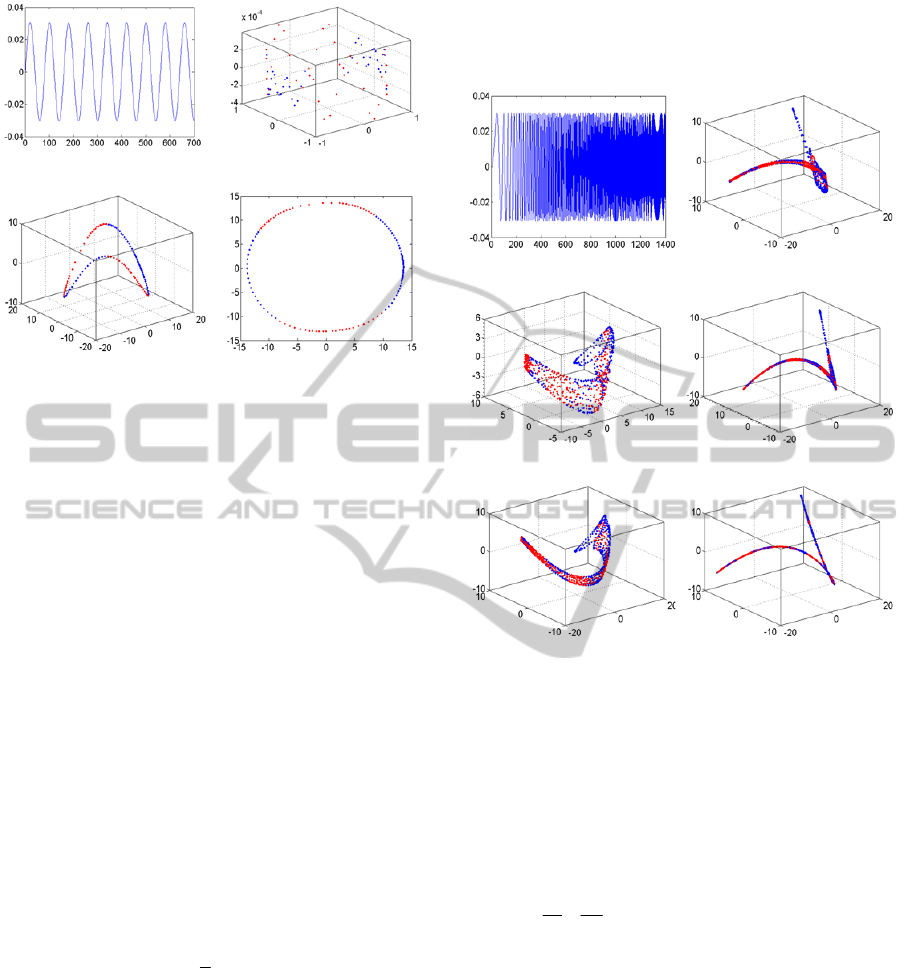
In Fig. 1, we show an example of the segment of
some sinusoidal signal, its PCA embedding and
commute time embedding. The segment is
composed of 700 samples, from which 676 patches
are extracted so that they may be maximally
overlapped. In this figure, patches of lower variance
are encoded with blue color, while patches of higher
variance with red color. Throughout this paper,
lower variance means it is less than the median of
the distribution of the variances over all patches in
the patch set, while higher variance is larger than the
median (Taylor, 2011). In PCA embedding, it is
meaningless to reduce their dimensionality into three
dimensional space, because the embedded points
corresponding to the patches are randomly scattered
around the three dimensional Euclidean space. It
means that one cannot effectively encode the patches
of 25 dimensional vectors into three dimensional
vectors, because the patches lie on the curved
manifold. However, the result of commute time
embedding shows that each patch is mapped densely
to generate a smooth curve inherent to the
characteristics of the signal and even two
dimensional space would be enough to represent
them without severe loss of inherent information.
Then, we investigate how the number of patches
in the patch set affects the embedding results. In
order to understand how many patches are needed
ICINCO2014-11thInternationalConferenceonInformaticsinControl,AutomationandRobotics
186
(a) (b)
(a) (b)
Figure 1: An embedding comparison between PCA and
commute time of a sinusoidal signal. (a) A sinusoidal
signal. (b) PCA embedding. (c) Commute time embedding
on three dimensional space. (d) Commute time embedding
on two dimensional space.
for the commute time embedding to have the
intrinsic geometry of smooth curve, we comprise
five patch sets, each of which is composed of
samples extracted from a chirp signal with varying
sample sizes of 700, 800, 900, 1,000, and 1,400. The
number of patches for each patch set is 676, 776,
876, 976, and 1,376, respectively. Fig. 2 depicts the
embedding of the patch sets associated with chirp
signals, whose numbers of patches are varied, using
the map given in Eq (5), where
3q
. When the
number of patches in the patch set is not sufficiently
enough compared with the statistics of the patches,
such as correlation among them, the distances
between pairs of patches are so randomly distributed
that some patches appear to be scattered on the
embedding subspace, while others are likely to be
aligned along a smooth curve. It is observed that the
embedding approaches its intrinsic geometry as the
number of patches increases.
Because the patches
n
x
extracted from the chirp
signal get to contain higher frequency components
as n increases, more patches are needed for smooth
and nearly continuous embedding compared with the
signal in Fig. 1, where the sinusoidal is periodic and
its patch set is sufficiently correlated. The commute
time embedding preserves commute time distance
between pairs of patches, which are equal to the
mutual Euclidean distance after embedding, so that
the distances between pairs of patches should be
more densely distributed in order to get the
continuous and smooth curve of embedding. That is
why the chirp signal needs more than 1,000 patches
for the embedding to be a smooth curve of inherent
geometry.
(a) (d)
(b) (e)
(c) (f)
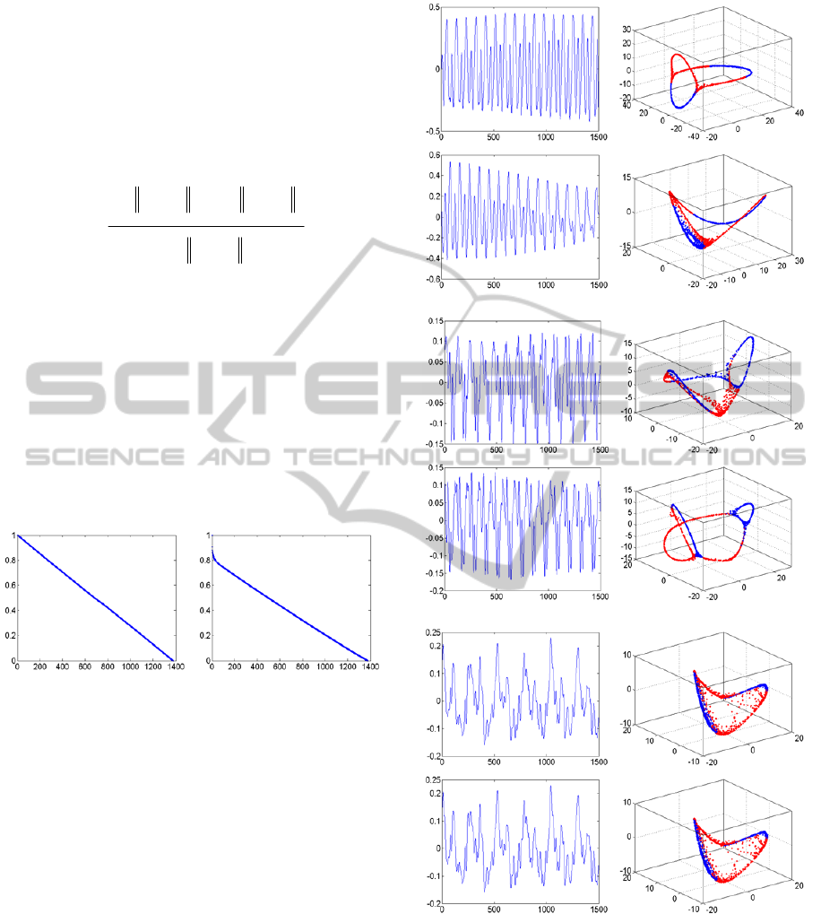
Figure 2: Evolution of a commute time embedding as the
number of patches extracted from a chirp signal increases.
(a) a chirp signal, The number of patches are (b) 676, (c)
776, (d) 876, (e) 976, (f) 1,376.
According to (von Luxburg et al, 2010), however,
the commute time
,cij
between pairs of nodes
i
v
and
j
v for all
ij
, converges to
11
ij
vol G
dd
as the number of nodes n
increases. This does not reflect connectivity of the
graph, just simply reflect the local degree
information only. Here,
,
u
v
dwuv
represents
a degree of a vertex
u
v
. It means that the time to hit
vertex
j
v
just depends on
j
d
if the number of
nodes gets large, regardless of which vertex
i
v
the
random walk starts from, and the random walk has
forgotten where it came from, by the time it is close
to vertex
j
v
. It is proved that this phenomenon
begins to happen even when the number of nodes
exceeds 1,000~2,000, depending on the statistics of
ManifoldEmbeddingbasedVisualizationofSignals
187
the patch set. Thus, we restrict the number of
patches should be less than 1,500, to avoid such
unwanted situations.
For the comparison purpose, we display in Fig. 3
the approximation errors of Laplacian eigenmap and
commute time embedding, when the chirp signal of
sample size of 1,400 is used. The approximation
error is defined as
22
,1 ,1
2
,1
NN
ij ij
ij ij
P
N
ij
ij
zz zz
eq
zz
(8)
In case of Laplacian eigenmap,
i
z
and
i
z
are
replaced with
i
y
and
i
y
, respectively, which are
defined in Eqs. (4)~(7). The approximation errors of
commute time embedding are less than those of the
Laplacian eigenmap, as shown in Fig. 3. It means
that scaling the entries of
i
z
by the inverse of the
eigenvalues of
sym
L
is tantamount to the effect of
more energy compaction in the process of
embedding, because it is expected the principal
components are more stressed.
(a) (b)
Figure 3: The approximation errors
P
eq
of (a)
Laplacian eigenmap and (b) commute time embedding.
4.2 Examples of Commute Time
Embedding
Based on some understanding of the manifold
embedding mentioned above, we assert that the
intrinsic geometries for the given waveform signals
can be generated using the manifold embedding.
Especially, graph Laplacian based embedding
algorithms are shown to generate low-dimensional
manifolds ( geometries of smooth curves ) given the
patch sets extracted from the waveform signals.
In order to capture the intrinsic geometries of the
musical instrumental sounds, we extract several
patch sets from each different segment of the
musical instrumental sounds – flutes, violins, cellos,
and speech signals – vowels [a:], [o:], [u;],
and then
embed them on the three dimensional Euclidean
(a)
(b)
(c)
Figure 4: Commute time embedding results of the musical
instrumental sounds. (a) flute, (b) violin, (c) cello.
space. It is shown in Fig. 4 some examples of
segments from which patch sets of instrumental
sounds are extracted and their corresponding
commute time embedding.
Flute sounds, as shown in Fig. 4-(a), are very
narrow-banded compared with those of violin or
ICINCO2014-11thInternationalConferenceonInformaticsinControl,AutomationandRobotics
188
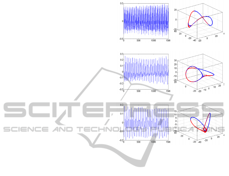
cello sounds, and their embeddings are composed of
two circles bounded. A close look at the figures
implies the number of circular shapes in the
embedding geometry is likely to be related to that of
dominant frequency components such as formants of
the waveforms. The waveforms are composed of
two dominant formants. The waveforms of violin
sounds, however, are more dynamic, i.e., have
couples of dominant frequency components,
compared with those of flutes, and are expected to
have more complicated geometric structures, as
shown in Fig. 4-(b). Indeed, the statistical
distribution of the patch sets extracted from the
different segments of the waveform varies according
to their spectral variations. For this reason, patch
sets, even though they are extracted from the same
waveform, may have quite different-looking
embedding. We get the similar results with the cello
sounds, which are displayed in Fig. 4-(c).
It is shown in Fig. 5 some examples of commute
time embedding of the patch sets extracted from the
segments of vowel sounds [a:], [o:] and [u;]. As
expected from the previous results, we observe the
embedding geometries similar to those of
instrumental sounds. The results given above
strongly support our earlier assertion that the
intrinsic geometries for the given waveform signals
can be generated using the graph Laplacian based
manifold embedding.
5 CONCLUSIONS
In this paper, we have explored the use of commute
time embedding for the purpose of transforming the
segments of some waveforms into their intrinsic
geometries. The embeddings corresponding to the
patch sets extracted from the dynamic regions of the
signals are scattered around some curves. We can
reduce such scatterings by smoothing the signals
from which patch sets are extracted, or increasing
the number of patches in the patch set. As long as
the segments of the waveforms are smooth enough
for the commute times between pairs of patches to
be densely distributed, it can be asserted that
commute time embedding generates their own
intrinsic geometries corresponding to the waveforms
on the embedding subspace. As a future research, we
would like to explore its application to pattern
classification or speech recognition in a geometric
way.
(a)
(b)
(c)
Figure 5: Commute time embedding results of the vowel
segments. (a) [a:], (b) [o:], (c) [u:].
REFERENCES
Belkin, M., Niyogi, P., 2003. Laplacian eigenmaps for
dimensionality reduction and data representation.
Neural Computation15(6), 1373-1396.
Brito, M., Chavez, E., Quiroz, A., Yukich, J., 1997.
Connectivity of the mutual k-nearest-neighbor graph in
clustering and outlier detection. Statistics and Probability
Letter.
Qiu, H., Hancock, E. R., 2007. Clustering and embedding
using commute times. IEEE Trans. PAMI, Vol. 29, No.
11, 1873-1890.
Roweis, S. T., Saul, L. K., 2000. Nonlinear dimensionality
reduction by locally linear embedding. Science
Vol.290, 2323-2326.
Taylor, K. M., 2011. The geometry of signal and image
patch-sets. PhD Thesis, University of Colorado,
Boulder, Dept. of Applied Mathematics.
Tenenbaum, J. B., deSilva, V., Langford, J. C., 2000. A
global geometric framework for nonlinear
dimensionality reduction. Science, Vol. 290, 2319-
2323.
von Luxburg, U., Radl, A., Hein, M., 2010. Getting lost in
space: Large sample analysis of the commute distance.
Neural Information Processing Systems.
ManifoldEmbeddingbasedVisualizationofSignals
189
