Object Contour Reconstruction using Bio-inspired Sensors

Christoph Will

, Joachim Steigenberger

and Carsten Behn

Department of Technical Mechanics, Technische Universit

at Ilmenau,

Max-Planck-Ring 12 (Building F), 98693 Ilmenau, Germany

Institute of Mathematics, Technische Universit

at Ilmenau, Weimarer Straße 25, 98693 Ilmenau, Germany

Keywords:

Vibrissa, Mechanical Contact, Beam, Bending, Large Deﬂections, Proﬁle Reconstruction.

Abstract:

This work is inspired and motivated by the sophisticated mammals sense organ of touch: vibrissa. Mammals,

especially rodents, use their vibrissae, located in the snout region – mystacial vibrissae – to determine object

contacts (passive mode) or to scan object surfaces (active mode). Here, we focus on the passive mode. In order

to get hints for an artiﬁcial sensing prototype, we set up a mechanical model in form of a long slim beam which

is one-sided clamped. We investigate in a purely analytical way a quasi-static sweep of the beam along a given

proﬁle, where we assume that the proﬁle boundary is strictly convex. This sweeping procedure shows up in

two phases, which have to be distinguished in proﬁle contact with the tip and tangentially contact (between tip

and base). The analysis eventuates in a phase decision criterion and in a formula for the contact point. These

are the main results. Moreover, based on the observables of the problem, i.e. the clamping moment and the

clamping forces, which are the only information the animal relies on, a reconstruction of the proﬁle is possible

– even with added uncertainty mimicking noise in experimental data.

1 INTRODUCTION

Rodents, like mice and rats, use tactile hairs in the

snout region (mystacial vibrissae) to obtain informa-

tion about the environment, whereby these vibrissae

are used in an active and passive mode. The vibris-

sae are supported in a compliant follicle sine complex

(FSC) as shown in Figure 1. The follicle sine com-

plex exhibits a large variety of mechanoreceptors, like

merkel cells, which detect the movement of the vib-

rissa base and convert this mechanical strain into sig-

nals to the central nervous system.

The main difﬁculty is the fact, that the animals get

only information about the environment from the pro-

cessing mechanoreceptors.

Inspired by this biological paragon and motivated

by its complex task to govern information, we focus

on a vibrissa in passive mode, i.e., object localiza-

tion. We set up a mechanical model in form of a plane

elastic bending rod for a quasi-static object scanning.

The exploitation of the corresponding mathematical

model is primarily not based on numerical methods,

but it relies on an analytical framework as far as pos-

sible. Before doing this, we focus on the state of art

to make a dissociation of the actual work in this ﬁeld.

nerve to CNS

blood

sinus

Merkel cell

Lancet

nerve ending

Paciniform

corpuscle

cirumferentially

oriented spiny

ending

vibrissal

shaft

Figure 1: Follicle sine complex (Behn, 2013b), arranged by

D. Voges (TU Ilmenau).

459

Will C., Steigenberger J. and Behn C..

Object Contour Reconstruction using Bio-inspired Sensors.

DOI: 10.5220/0005018004590467

In Proceedings of the 11th International Conference on Informatics in Control, Automation and Robotics (ICINCO-2014), pages 459-467

ISBN: 978-989-758-039-0

 2014 SCITEPRESS (Science and Technology Publications, Lda.)

2 STATE OF THE ART

Various approaches are done in literature to model

the biological paragon to get hints for a technical

implementation in, e.g., robotics for obstacle detec-

tion (Kim and M

oller, 2006), (Pearson et al., 2011),

(Prescott et al., 2009).

First models, like the one presented in (Hirose

et al., 1989), consider long thin elastic beams for de-

tection of deformation caused by an obstacle contact.

If this “whisker-like” sensor perceives a deformation

of the beam (which has to be sufﬁciently large as to

exceed some given threshold), the actual position is

marked for further trajectory planning. Hence, the

pure existence of an obstacle is needed, no other in-

formation about the obstacle is requested (just detec-

tion).

Further approaches are given in (Kim and M

oller,

2007) and (Tuna et al., 2012), which realize additional

information about the obstacle. In (Tuna et al., 2012),

a contact point with an obstacle is estimated using the

angle of deﬂection at the base (inspired by methods

in computer tomography, ray deﬂection). The authors

in (Kim and M

oller, 2007) use the linear theory of

elasticity in application to large deﬂections of a beam.

In both methods, only the angle of deﬂection, neither

forces nor moments, are measured.

In (Birdwell et al., 2007), another model is given

which incorporates both small deformations and the

pre-curvature of the beam. This is done in adding the

pre-curvature to the linear deﬂection of the beam to

get the actual position of the beam. The achievable

accuracy of the model depends on the pre-curvature

of the beam, because the curvature is assumed to be

a function on the beam axis. For small radii of suf-

ﬁciently long beams, this method can fail due to the

cartesian coordinate system. Also, it is still unclear, if

the pre-curvature of the vibrissa results in a pre-stress.

An improved method for object localization and

shape detection is proposed in (Scholz and Rahn,

2004) for plane problems, in (Clements and Rahn,

2006) for spatial problems. In both works, the au-

thors switch from linear approximation of the curva-

ture to the description of the problem in natural coor-

dinates. This is a main improvement in comparison

to works presented above. Thus, they allow for large

deﬂections of the beam, which results in a clear for-

mulation of the boundary conditions. Further, exper-

imental data are used in a numerical reconstruction

algorithm in Simulink which results in the deformed

beam shapes and a numerical values for the contact

point. The entirety of all these beam shapes models

the shape of the object geometry.

Recent works, like (Pammer et al., 2013), approx-

imate the curvature of the beam in using ﬁnite differ-

ences. This gives the possibility to consider the curva-

tures of an undeformed vibrissa, but analytical equa-

tions with new insights do not exist due to numerical

simulations.

3 AIM AND SCOPE

In this paper, due to Section 2, we focus on an entire

analytical treatment of the scanning problem of an ob-

stacle via a beam vibrissa. Since we have to allow for

large deﬂections of the beam, we introduce the non-

linear Euler-Bernoulli theory of beam bending. More-

over, we set up a mechanical model and investigate

the quasi-static bending behavior, when the beam is

swept along an obstacle. In order to get information

about the obstacle, we determine both forces and mo-

ments at the base (here: a clamping of the beam) as

solutions of a boundary value problem (BVP). Re-

versely, we use them in an initial value problem (IVP)

to determine a contact point of the deformed beam

with the obstacle. The series of all contact points ex-

hibit the shape of the obstacle.

4 MODELING

The present paper deals with the problem what an an-

imal “feels” and perceives by means of a single vib-

rissa while moving along an obstacle, and which in-

formation it can get about the obstacle. As already

mentioned in Section 1, the only information is avail-

able at the support of the vibrissa.

4.1 Assumptions

In order to get further information, we treat the prob-

lem analytically to the greatest extent. The work is

based on (Steigenberger, 2013) and (Will, 2013). In

order to model the problem, the following assump-

tions are made:

• The problem is treated as a quasi-static one.

• We restrict the problem to an (x, y)-plane. The

(originally undeformed) vibrissa is vertical, its

base moves along the x-axis from the right to the

left.

• The vibrissa is assumed as a long, slim, straight

(until now, no pre-curvature is assumed) beam

with constant second moment of area I

, constant

Young’s modulus E and length L. Thus, ignoring

shear stress, the Euler-Bernoulli theory for large

deﬂections is applicable.

ICINCO2014-11thInternationalConferenceonInformaticsinControl,AutomationandRobotics

460

• The stress of the beam is sufﬁciently small to use

Hooke’s law of linear elasticity.

• The support of the beam is a clamp.

Clearly, this does not match the reality of the vib-

rissa. In further works, we take a glimpse to an

elastic support due to the compliant properties of

the FSC, see Figure 1.

• The obstacle contour (i.e., its boundary) is a

strictly convex function g : x 7→ g(x), with g ∈

(R;R).

• The object contact is ideal, i.e., the deformation

of the beam is caused by a single contact force

perpendicular to the obstacle proﬁle. Friction is

not taken into account.

4.2 Model

The starting point is

κ(s) =

(s)

, (1)

which is valid due to the assumptions in Section 4.1.

Here, M

(·) denotes the bending moment with re-

spect to the z-axis, s ∈ [0, L] is the arc length of the

beam, and κ(·) represents the curvatures, see Figure

2. For the sake of brevity, we introduce dimension-

less variables. The units of measure are [length] = L,

[moments] = EI

−1

and [forces] = EI

−2

(for ex-

ample: s = Ls

∗

, s

∗

∈ [0, 1]).

E, I

, L

ϕ(s)

force

Figure 2: Euler-Bernoulli beam under large deﬂection.

As from now, all quantities are given in di-

mensionless representation, whereby the asterisk is

dropped. Then, (1) becomes

κ(s) = M

(s) (2)

and the deformed beam is described by

x(s) = cos(ϕ(s)) ,

y(s) = sin (ϕ(s)) ,

ϕ(s) = κ(s) ,











with initial conditions x(0) = x

, y(0) = 0 and

ϕ(0) =

(due to the clamping). Because of the strict

convexity of g, x and y are functions of the slope angle

α:

g(x) = g

(x) = tan(α)

⇒ x = ξ(α)

= g

0−1

(tan(α)),

⇒ y = η(α)

= g(ξ(α)).

Now:



x, g(x)



7→



ξ(α), η(α)



To formulate the boundary conditions, we have to dis-

tinguish two conﬁgurations of contacting the proﬁle,

see Figure 3:

• Phase A: Contact of beam tip and proﬁle with

ϕ(1) ≥ α,

• Phase B: Contact of a point s

∈ (0, 1) and the

proﬁle with equal angles ϕ(s

) = α.

−2 −1 0 1 2

0.5

(ξ(α), η(α))

Tip contact and deformed beams in phase A

Deformed beam in phase B

Phase change

Legend:

Figure 3: Proﬁle with deﬂected beams.

In both phases, the contact point is given by the slope

angle α of the proﬁle.

ObjectContourReconstructionusingBio-inspiredSensors

461

1.6

1.8 2 2.2 2.4

0.5

#„

Figure 4: Deﬂected beam in Phase A.

4.3 Phase A: Contact at the Tip

Using Figure 4, the bending moment is for s ∈ (0, 1):

(s) = f





y(s) −η(α)



sin(α)



x(s) −ξ(α)



cos(α)



(3)

Decoupling of the bending moment from x(s) and

y(s), the derivative of (3) yields the following ODE

system (4) with boundary conditions (5):

(a) κ

(s) = f cos(ϕ(s) −α)

(b) ϕ

(s) = κ(s)

(s) = cos(ϕ(s))

(d) y

(s) = sin(ϕ(s))

(4)

(a) ϕ(0) =

(b) y(0) = 0

(d) x(1) = ξ(α)

(e) y(1) = η(α)

(5)

This BVP splits into two separate problems:

{(4a,b),(5a,c)} and {(4c,d),(5b,d,e)}. The ﬁrst one

has

= 2 f (sin(ϕ −α) −sin(ϕ

−α)) (6a)

= 4 f sin



ϕ −ϕ



cos



ϕ + ϕ

−2α



. (6b)

as a ﬁrst integral with ϕ

= ϕ(1).

Remark 4.1. The bending moment, considering the

lower part of the beam, depends on the clamp reac-

tions M

, F

, which results in a ﬁrst integral of

the form:

= 2 f sin(ϕ −α)−2 f cos(α) + M

Because κ

(s) ≥ 0 has to be fulﬁlled, three cases

have to be discussed for (6b) with f > 0:

1. At least one factor is zero: hence κ(s) ≡ 0, and

the beam is not deformed at all.

2. Both factors are negative: The sine function is

positive on the interval (−π, 0) and negative on

(π, 2π). This results in the inequations

−2π < ϕ(s) −ϕ

< 0 ∨ 2π < ϕ(s) −ϕ

< 4π.

Hence ϕ(s) < ϕ

∨ ϕ(s) > 2π. This is a contra-

diction, because ϕ(s) ∈





∀s ∈ [0, 1].

3. Both factors are positive: The sine function is pos-

itive on the domain (0, π), the cosine function on



−



. Therefore, it must hold:

0 < ϕ(s) −ϕ

< 2π ∧ −π < ϕ(s) + ϕ

−2α < π .

The ﬁrst inequality contains no additional infor-

mation, the second one yields:

ϕ(s) + ϕ

< π + 2α ∀s

⇒ ϕ

+ 2α, since ϕ(s) ≤

Therefore, the angle ϕ

has to be in the domain

α < ϕ

< min



+ 2α



Due to the assumptions, the curvature is non-

positive along the solutions of (4a,b), which results

in, using (6a):

dϕ(s)

= κ(s)

=−

2 f (sin(ϕ(s) −α) −sin(ϕ

−α)) (7)

as a ODE with separated variables for ϕ(s). Introduc-

ing H

: (t, u) 7→ F

sin



−



sin



−



, sin



−



, (8)

where F is the incomplete elliptic integral of ﬁrst kind

according to the deﬁnition (Abramowitz and Stegun,

1972, 17.2.7)

F : (z, k) 7→

1 −ψ

1 −k

dψ,

the separation of variables applied on (7) with initial

value (5a) yields:

f s = H



ϕ(s) −α, ϕ

−α



−H



−α, ϕ

−α



(9)

Hence, the contact force f can be expressed as

f (ϕ

, α)



(ϕ

−α, ϕ

−α)

−H



−α, ϕ

−α





(10)

Now, the only unknown parameter at this stage is the

angle ϕ

at the tip. To determine this parameter, (5b,e)

have to be used in the following two ways.

ICINCO2014-11thInternationalConferenceonInformaticsinControl,AutomationandRobotics

462

4.3.1 Substitution of Variable

Here, y is given in dependence on ϕ:

dy(s)

dϕ(s)

dy(ϕ)

dϕ

κ(ϕ)

sin(ϕ) ,

with boundary conditions y(

) = 0 and y(ϕ

) = η(α).

At ﬁrst, the ﬁrst condition leads to

y(ϕ) = −

√

2 f

sin(τ)

sin(τ −α) −sin(ϕ

−α)

dτ.

The second boundary condition results in an implicit

expression for ϕ

∈



α, min



+ 2α





η(α)

2 f +

sin(τ)

sin(τ −α) −sin(ϕ

−α)

= 0.

(11)

Note that the integral (11) can be represented by

means of elliptic integrals and solved for ϕ

4.3.2 Shooting Method

Instead of substituting the variable, the problem can

efﬁciently be solved by applying a shooting method

for ϕ

, which can be both faster and more accurate.

Let ϕ

∗

∈



α + ε, min



+ 2α



−ε



be a valid

candidate for ϕ

. The corresponding deﬂection angle

ϕ(s) can be calculated from (9) using (10):

ϕ(s, ϕ

∗

) = α + H

−1



f (ϕ

∗

, α)s



−α, ϕ

∗

−α



, ϕ

∗

−α



with

−1

(t, u)

= −

+ 2 arccos



JacobiSN



cos





cos







from (8) and JacobiSN according to (Abramowitz and

Stegun, 1972, 16.1.3 and 16.1.5).

Now (4d) with (5b) yield

y(s, ϕ

∗

) =

sin(ϕ(τ, ϕ

∗

))dτ,

which can be numerically computed. The shooting

value for ϕ

∗

is correct, if y(1, ϕ

∗

) −η(α) = 0.

0 0.2 0.4

0.6

0.8 1 1.2

0.1

0.2

0.3

0.4

#„

Figure 5: Deﬂected beam in Phase B, contact s

∈ (0, 1).

Summarizing, independent of the chosen method,

is now known. The solution of (4c,d) is:

x = ξ(α) +

cos(ϕ(τ))dτ, (12)

y = η(α) +

sin(ϕ(τ))dτ.

4.4 Phase B: Tangential Contact

The bending moment is now, with yet unknown con-

tact point s

(see Figure 5):

(s) =















y(s) −η(α)



sin(α)



x(s) −ξ(α)



cos(α)



, s ∈ (0, s

]

0 , s ∈ (s

, 1).

(13)

The related BVP with s ∈ (0, s

) is:

(a) κ

(s) = f cos(ϕ(s) −α)

(b) ϕ

(s) = κ(s)

(s) = cos(ϕ(s))

(d) y

(s) = sin(ϕ(s))

(14)

(a) ϕ(0) =

(b) y(0) = 0

) = 0

(d) ϕ(s

) = α

(e) x(s

) = ξ(α)

(f) y(s

) = η(α)

(15)

A ﬁrst integral of (14a) together with (14b) and

(15c) is

= 2 f sin(ϕ −α)

⇒

ϕ(s) = κ(s) = −

2 f

sin(ϕ(s) −α).

(16)

ObjectContourReconstructionusingBio-inspiredSensors

463

Equation (14b) with (16) and (15a) yield

f s = H

(ϕ(s) −α) −H



−α



which can be solved for ϕ(s):

ϕ(s) = α + H

−1



f s + H



−α



using

: t → F

√

2sin



−



√

with

−1

(t)=−

+ 2 arccos

√

JacobiSN

√

Since ϕ(s

) = α is known, the contact force can be

expressed as

f =

(0) −H



−α



. (17)

Again, considering the function y to get the last

missing parameter s

, condition (15b) results in:

y(s) =

√

f s+H

(

−α

)

(

−α

)

sin



α + H

−1

(τ)



dτ. (18)

Summarizing, (17), (18) and (15f) yield

f (α) =







η(α)

(0)

(

−α

)

sin



α + H

−1

(τ)



dτ







(19)

Now, (17) and (19) lead to the following equation

for the contact point s

(α) =

η(α)



(0) −H



−α



(0)

(

−α

)

sin



α + H

−1

(τ)



dτ

. (20)

The last integral of (14c) with (15e) is:

x(s) = x

√

f s+H

(

−α

)

(

−α

)

cos



α + H

−1

(τ)



dτ,

whence, with s = s

, we obtain the foot coordinate

= ξ(α) −

√

(0)

(

−α

)

cos



α + H

−1

(τ)



. (21)

Finally, for both phases, the footpoint x

is derived

using (12) and (21). Using (10) and (19) we can deter-

mine f and, hence, knowing α, also the contact force

#„

F . With f we get the clamping forces F

and F

, as

well as the clamping moment M

using (3) and (13).

5 SIMULATIONS

Let us focus on the following two proﬁle functions:

: x 7→

(

−

√

−x

, x > 0 ,

−

−x

+ 1, else.

Function g

is a parabola, and g

is a proﬁle composed

of two circles, both shown in Figure 6.

−1.5

−1

−0.5

0.5

1.5

0.5

(a) Parabola proﬁle g

−1.5

−1

−0.5

0.5

1.5

0.5

(b) Proﬁle composed of two circles g

Figure 6: Proﬁles under consideration.

Computed observables for proﬁle g

are exem-

plarily shown in Figure 7.

−1.5

−1

−0.5

0.5

1.5

(a) Clamping moment M

(maximum marked with )

−1.5

−1

−0.5

0.5

1.5

(b) Clamping forces F

( F

; F

)

Figure 7: Observables with proﬁle function g

. marks the

change between Phase A and Phase B.

ICINCO2014-11thInternationalConferenceonInformaticsinControl,AutomationandRobotics

464

The maximum clamping moment occurs in Phase

B, but besides a change of phase in M

and F

. Ob-

viously, no direct information about the obstacle can

be extracted directly from the curve of the observ-

ables. We rather use the computed observables for

an object proﬁle reconstruction in the next section.

6 RECONSTRUCTION OF THE

PROFILE

At this stage, we have the observables x

, F

, M

(values which are assumed that an animal can solely

rely on) numerically computed at hand. They repre-

sent the only information. In experiments these values

are produced by a measurement device.

We have to focus on a reconstruction procedure of

the obstacle proﬁle, out of these “measured” values.

6.1 Analysis

Let us start with the following information at the base:

κ(0) = lim

s→0+

(s) = −M

ϕ(0) =

x(0) = x

y(0) = 0

and

α = −arctan





, f =

+ F

The main difﬁculty is to decide which phase the

beam actually undergoes. To solve this, let us focus

on the curvature (in Phase A, Phase B, or somewhere):

Ph. A: κ

(s) = 2 f (sin(ϕ(s) −α) −sin(ϕ

−α)) ,

(22)

any s: κ

(s) = 2 f (sin(ϕ(s) −α) −cos(α)) + M

(23)

Ph. B: κ

(s) = 2 f sin(ϕ(s) −α). (24)

Obviously, it is Phase B iff ϕ

= α. Using (23), ϕ

can be determined by:

= α −arcsin

−2 f cos(α)

2 f

which results in the decision condition for Phase B

with only known parameters:

−2F

= 0. (25)

If (25) is valid, the contact force is applied at s

∈

(0, 1) which can be computed:

(0) −H



−α



√

Else, if (25) does not hold, the contact force is applied

at s

= 1.

Now, the IVP is solved numerically using MAT-

LAB’s variable order Adams-Bashforth-Moulton

PECE solver:

(s) = −

2 f sin(ϕ(s) −α)−2 f cos(α) +M

ϕ(0) =

(s) = cos(ϕ(s)) , x(0) = x

(s) = sin(ϕ(s)) , y(0) = 0,

which results in the reconstructed contact point:

ξ(α) = x(s

), η(α) = y(s

6.2 Numerics

During reconstruction, the error for each component

point k along the proﬁle function g, shown in Figure 8,

is computed using the euclidian norm of the distance

between the given and the reconstructed contact point:

error





)



−



ξ(α

)

η(α

)





with s

as reconstructed contact point, (x

(s), y

(s))

the reconstructed position of the beam in the plane

and (ξ(α

), η(α

)) the given contact point for com-

puting the observables.

−1.5

−1

−0.5

0.5

1.5

0.2

0.4

0.6

0.8

·10

−6

error

(a) Parabola proﬁle g

−1.5

−1

−0.5

0.5

1.5

0.2

0.4

0.6

0.8

·10

−6

error

(b) Proﬁle g

Figure 8: Reconstruction errors.

ObjectContourReconstructionusingBio-inspiredSensors

465

−1.2 −1 −0.8

−0.6

−0.4 −0.2 0 0.2 0.4

0.6

0.8 1

0.5

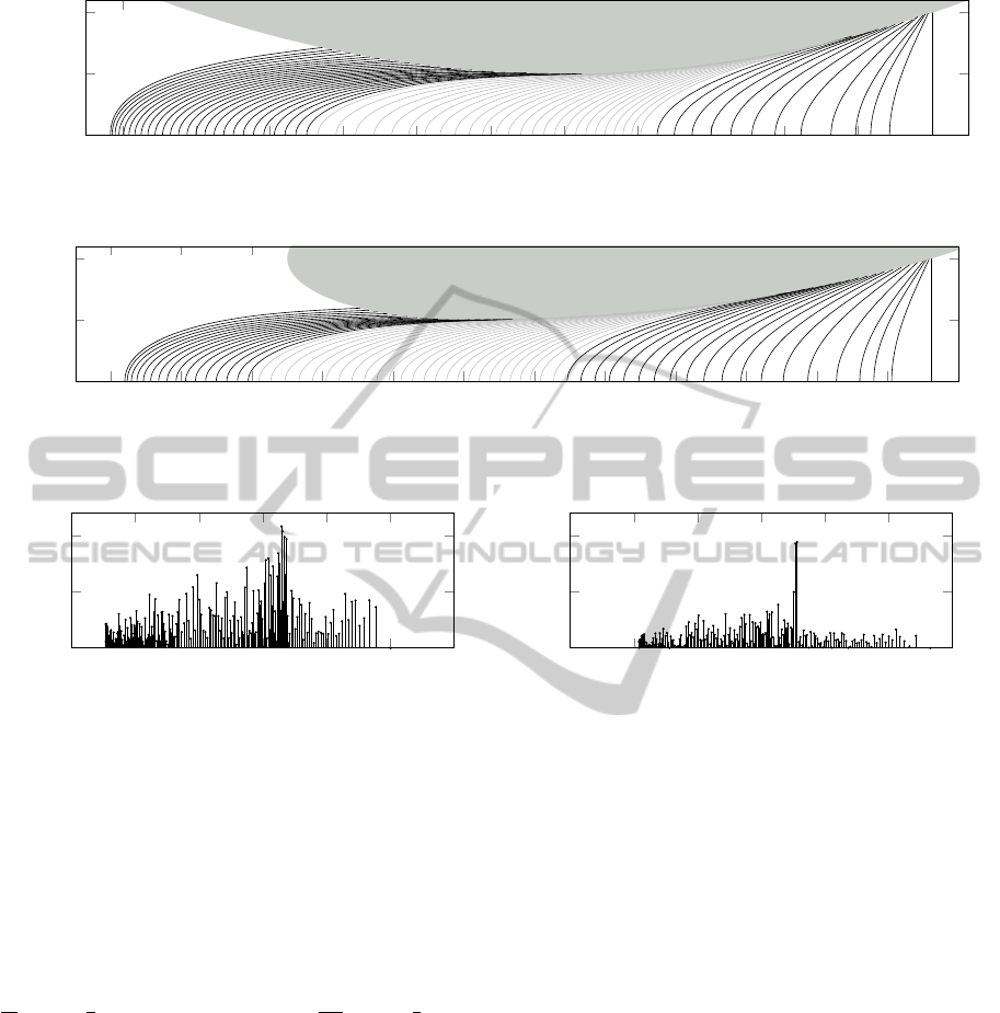
(a) Sweep along proﬁle g

−1 −0.8

−0.6

−0.4 −0.2 0 0.2 0.4

0.6

0.8 1 1.2 1.4

0.5

(b) Sweep along proﬁle g

−1.5

−1

−0.5

0.5

1.5

0.5

·10

−2

error

−1.5

−1

−0.5

0.5

1.5

0.5

·10

−2

error

(d) Reconstruction error for proﬁle g

Figure 9: Reconstruction with added noise.

6.3 Reconstruction under Uncertainties

Because of lack of experiments, we assume that the

computed observables underlie some measurement

noise like in real experiments. To generate some noise

to the observables, random uncertainty is added to

, F

and M

. The scale of the added values is



rnd −



for forces F

, F

and

100



rnd −



for

moment M

, rnd ∈(0, 1) according to technical data

sheet of a Schunk GmbH & Co. KG FT-Mini-40 force

and moment sensor.

Besides the error obtained by the noisy observ-

ables, the decision if a tuple of observables belongs to

Phase B or Phase A using (25) is very critical in the

process of reconstruction. During the reconstruction

using the computed observables,



−2F



≤10

−4

was used as condition for Phase B. With the added

values, a higher tolerance gives better results, thus



−2F



≤ 0.08 was used. As shown in Figure

9(c) and (d), the reconstruction error is increased by

four orders of magnitude if noise is added. For prac-

tical application, the proﬁle is still sufﬁciently recon-

structed as shown in Figure 9.

Clearly, the shape of the deformed vibrissa is an

important part of the theory, but of little relevance in

the result of the practical reconstruction process. The

only important result is the sequence of the computed,

reconstructed contact points of the proﬁle.

7 CONCLUSION

Analytical investigations have shown that it is pos-

sible to reconstruct a proﬁle contour by one single

sweep of a thin elastic Euler-Bernoulli beam along it.

As a typical ﬁrst step in modeling we determined

the “observables” (reactions of the clamping), which

an animal relies solely on, in a purely analytical way

because of lack of experiments, in contrast to (Scholz

and Rahn, 2004). But, the theoretical results showed

up a single equation for a decision of the contact be-

havior of the beam with the object: contact at the tip,

or contact between base and tip. This decision is new

in literature and provides an easier and faster com-

ICINCO2014-11thInternationalConferenceonInformaticsinControl,AutomationandRobotics

466

putation of the deformed vibrissa and reconstruction

of the proﬁle as well. Furthermore, an explicit an-

alytical formula to determine the contact point out of

the “measured” values of the observables was derived.

Both will increase the efﬁciency in experiments in fu-

ture.

These results were obtained without assuming any

estimation or approximation of describing functions.

This is rather new in literature, in contrast to (Kim and

oller, 2007), (Birdwell et al., 2007).

Further on, to mimick experimental data, a re-

construction based solely on the “observables” with

added random noise (uncertainty — mimicking noise

in experiments) is valid for various proﬁles. But, ob-

viously, the contact point approximation accuracy di-

minished from 10

−6

to 10

−2

(dimensionless), i.e., if

the vibrissa is 1 m long then the obstacle contact po-

sition can be determined in the plane with an accu-

racy of 1 cm by a single measuring point during ob-

stacle contour sensing. These results maintain the

hypothesis from biologists, that animals can navigate

by strongly relying on their mechanoreceptors at the

FSC.

Near future (theoretical) work is addressed to the

following investigations:

• analysis of the inﬂuence of an elastic support as in

the biological paragon (Behn, 2013a): This could

be needed to guarantee a bounded bending mo-

ment in controlling the support stiffness (i.e., the

vibrissa does not brake during sensing – just think

about a cat passing a fence).

• investigations on non-strictly convex proﬁles:

There can appear ﬂat points and we have to ad-

just our theory.

• switching from investigations in the vertical x-y-

plane to a 3-dimensional sensing problem.

Intermediate future (experimental) work is addressed

to experiments. At present, we are working on a de-

sign of a prototype for sensing obstacles.

Far future work is addressed to an application of

such tactile sensors to mobile robotics (or a mouse-

like robot) for online object localization and different

tasks similar to the prototypes presented in (Kim and

oller, 2006) and (Pearson et al., 2011).

REFERENCES

Abramowitz, M. and Stegun, I. A. (1972). Handbook

of mathematical functions: With formulas, graphs,

and mathematical tables, volume 55 of National Bu-

reau of Standards applied mathematics series. United

States Department of Commerce, Washington, DC,

10. print., dec. 1972, with corr edition.

Behn, C. (2013a). Mathematical Modeling and Control of

Biologically Inspired Uncertain Motion Systems with

Adaptive Features. PhD thesis, Technische Univer-

sit

at Ilmenau, Ilmenau.

Behn, C. (2013b). Modeling the behavior of hair follicle

receptors as technical sensors using adaptive control.

In ICINCO (1), pages 336–345.

Birdwell, J. A., Solomon, J. H., Thajchayapong, M., Taylor,

M. A., Cheely, M., Towal, R. B., Conradt, J., and Hart-

mann, M. J. Z. (2007). Biomechanical Models for Ra-

dial Distance Determination by the Rat Vibrissal Sys-

tem. Journal of Neurophysiology, 98(4):2439–2455.

Clements, T. N. and Rahn, C. D. (2006). Three-dimensional

contact imaging with an actuated whisker. IEEE

Transactions on Robotics, 22(4):844–848.

Hirose, S., Inoue, S., and Yoneda, K. (1989). The whisker

sensor and the transmission of multiple sensor signals.

Advanced Robotics, 4(2):105–117.

Kim, D. and M

oller, R. (2006). Passive sensing and active

sensing of a biomimetic whisker. In Rocha, L. M.,

editor, Artiﬁcial life X, A Bradford book, pages 282–

288. MIT Press, Cambridge, Mass.

Kim, D. and M

oller, R. (2007). Biomimetic whiskers for

shape recognition. Robotics and Autonomous Systems,

55(3):229–243.

Pammer, L., O’Connor, D. H., Hires, S. A., Clack, N. G.,

Huber, D., Myers, E. W., and Svoboda, K. (2013).

The mechanical variables underlying object localiza-

tion along the axis of the whisker. The Journal of

neuroscience : the ofﬁcial journal of the Society for

Neuroscience, 33(16):6726–6741.

Pearson, M. J., Mitchinson, B., Sullivan, J. C., Pipe,

A. G., and Prescott, T. J. (2011). Biomimetic vib-

rissal sensing for robots. Philosophical Transac-

tions of the Royal Society B: Biological Sciences,

366(1581):3085–3096.

Prescott, T., Pearson, M., Mitchinson, B., Sullivan, J.

C. W., and Pipe, A. (2009). Whisking with robots:

From Rat Vibrissae to Biomimetic Technology for Ac-

tive Touch. IEEE Robotics & Automation Magazine,

16(3):42–50.

Scholz, G. R. and Rahn, C. D. (2004). Proﬁle Sensing With

an Actuated Whisker. IEEE Transactions on Robotics

and Automation, 20(1):124–127.

Steigenberger, J. (2013). A continuum model of passive

vibrissae.

Tuna, C., Solomon, J. H., Jones, D. L., and Hartmann, M.

J. Z. (2012). Object shape recognition with artiﬁcial

whiskers using tomographic reconstruction. In IEEE

International Conference on Acoustics, Speech and

Signal Processing (ICASSP), pages 2537–2540, Pis-

cataway, NJ. IEEE.

Will, C. (2013). Anwendung nichtlinearer Biegetheorie

auf elastische Balken zur Objektabtastung am Beispiel

passiver Vibrissen mit unterschiedlicher Lagerung

(Application of non-linear beam theory for obstacle

detection with respect to the biological paragon of a

passive vibrissa using different supports). Master the-

sis, Technische Universit

at Ilmenau, Ilmenau.

ObjectContourReconstructionusingBio-inspiredSensors

467