
Collaborative Kalman Filtration
Bayesian Perspective
Kamil Dedecius
Institute of Information Theory and Automation, Academy of Sciences of the Czech Republic
Pod Vod
´
arenskou v
ˇ
e
ˇ
z
´
ı 4, 182 08 Prague, Czech Republic
Keywords:
Bayesian analysis, Estimation Theory, Distributed estimation, Kalman filter.
Abstract:
The contribution studies the problem of collaborative Kalman filtering over distributed networks with or with-
out a fusion center from the theoretically consistent Bayesian perspective. After presenting the Bayesian
derivation of the basic Kalman filter, we develop a versatile method allowing exchange of observations among
the network nodes and their local incorporation. A probabilistic nodes selection technique based on prior
knowledge of nodes performance is proposed to reduce the communication requirements.
1 INTRODUCTION
The theory of distributed parameter estimation has at-
tained tremendous attention in the last decade, par-
ticularly due to still cheaper and increasingly pow-
erful (wireless) sensor networks. According to the
network topology, three main types of networks and
hence algorithms can be distinguished. First, the net-
works with a fusion center, responsible for informa-
tion processing. In these networks, the nodes do not
necessarily evaluate any modelling/estimation. Sec-
ond, the networks with a Hamiltonian cycle, similar
to the token ring computer networks. There exists
only one path in these networks; the information cir-
culates in the network and the nodes incorporate own
information (observations) into it. Third, the diffu-
sion networks, avoiding both the fusion center and
the Hamiltonian cycle. These networks with a higher
degree of connectedness employ cooperation among
nodes within subsets called neighborhoods. The other
two topology types can be viewed as highly degraded
diffusion networks. Unlike them, the (non-degraded)
diffusion networks have the highest robustness due
to the avoidance of single points of failure (SPOFs).
Therefore, we focus on filtering in diffusion networks,
while keeping in mind that the centralized and Hamil-
tonian types can be solved with the proposed results
as well.
Distributed Kalman filtering we focus on is
closely related to the distributed recursive least
squares, first proposed for the diffusion networks in
(Cattivelli et al., 2008) in the classical paradigm and
in (Dedecius and Se
ˇ
ck
´
arov
´
a, 2013) from the Bayesian
point of view. For a totally connected (hence decen-
tralized) network, the Kalman filter was proposed by
(Speyer, 1978; Ribeiro et al., 2006). However, the
requirement of total connectedness is relatively pro-
hibitive. Three types of the consensus Kalman fil-
ters, avoiding this requirement, were proposed, e.g.,
in the seminal paper (Olfati-Saber, 2007). These so-
lutions rely on the so-called microfilter architecture.
The consensus algorithms typically impose the need
of intermediate averaging iterations among nodes, de-
manding additional in-network communication. The
diffusion Kalman filter, (Cattivelli and Sayed, 2010),
avoids them.
The main problem associated with distributed
estimation is the communication burden. Several
strategies for its alleviation were proposed, however,
mostly for centralized networks. For example, (Gupta
et al., 2006) considers the case where only one node
can take measurements at a time and proposes a
stochastic scheme for its selection. Another, also cen-
tralized scheme, was proposed in (Mo et al., 2006),
with the goal of minimizing an objective function re-
lated to the Kalman filter error covariance matrix. The
most recent distributed solution (Yang et al., 2014)
considers minimization of the mean square estimation
error.
The purpose of this paper is twofold: first, we re-
view the formal derivation of the Kalman filter as-
similating measurements obtained from the network
(or its part), given in a detail in (Dedecius, 2014).
This derivation follows the basic Bayesian approach
468
Dedecius K..
Collaborative Kalman Filtration - Bayesian Perspective.
DOI: 10.5220/0005018104680474
In Proceedings of the 11th International Conference on Informatics in Control, Automation and Robotics (ICINCO-2014), pages 468-474
ISBN: 978-989-758-039-0
Copyright
c
2014 SCITEPRESS (Science and Technology Publications, Lda.)

to the Kalman filter, e.g. (Meinhold and Singpur-
walla, 1983) or (Peterka, 1981). Second, and more
importantly, a probabilistic method for selection of
a subset of network nodes is developed, that allows
to significantly reduce the communication resources.
This contribution focuses on the measurements in-
corporation only. The state-of-art methods often in-
volve a step when the resulting estimates are merged
as well. We leave the probabilistic selection of net-
work nodes for merging as the future work.
2 KALMAN FILTER: BAYESIAN
FORMULATION
Consider a system with an observable real multivari-
ate output y
t
linearly dependent on multivariate latent
system state x
t
and, if present, a known multivariate
input (control) u
t
. Suppose, that the system is de-
scribed by the state-space model
x
t
= Ax
t−1
+ Bu
t
+ w
t
y
t
= Cx
t
+ e
t
,
where A, B and C are known matrices of appropriate
dimensions and the mutually independent noise vari-
ables
w
t
∼ N (0, R
w
)
e
t
∼ N (0, R
e
).
From the Bayesian viewpoint, the state variable
x
t
is a model parameter with the probability density
function (pdf) p(x
t
|x
t−1
, u
t
) given by
N (A ˆx
t−1
+ Bu
t
, R
w
), (1)
while the output y
t
obeys the model
y
t
|x
t
∼ N (C ˆx
t
, R
e
) (2)
.
Denote ˆx
t−1
and P
t−1
the mean and covari-
ance of the state given past observations X
t−1
=
{x
0
, x
1
, . . . , x
t−1
} and U
t
= {u
0
, . . . , u
t
}
x
t−1
|U
t−1
, Y
t−1
∼ N (ˆx
t−1
, P
t−1
).
The state prediction follows from (1) and (2) using the
chain rule and marginalization
p(x
t
|U
t
, Y
t−1
)
=
Z
p(x
t
|x
t−1
, u
t
)p(x
t−1
|U
t−1
, Y
t−1
)dx
t−1
, (3)
yielding a conditional distribution for x
t
x
t
|U
t
, Y
t−1
∼ N (A ˆx
t−1
+ Bu
t
, AP
t−1
A
|
+ R
w
). (4)
We adopt the convention to denote the predicted co-
variance by P
−
t
,
P
−
t
= AP
t−1
A
|
+ R
w
.
Similarly, we denote
ˆx
−
t
= A ˆx
t−1
+ Bu
t
.
The Bayesian estimation of x
t
given observations
Y
t
and U
t
incorporates the latest observation y
t
into the
prior pdf p(x
t
|U
t
, Y
t−1
) via the Bayes’ theorem
p(x
t
|U
t
, Y
t
) ∝ p(y
t
|x
t
)p(x
t
|U
t
, Y
t−1
), (5)
where ∝ denotes proportionality, i.e., equality up to a
normalizing constant.
The posterior pdf in (5) is proportional to a prod-
uct of two normal pdfs with known variances, hence
again a normal pdf. The exponent from the product
reads
−
1
2
(y
t
−C ˆx
−
t
)
|
R
−1
e
(y
t
−C ˆx
−
t
)
+(x
t
− ˆx
t
)
|
P
−
t
(x
t
− ˆx
t
)
After completion of squares we conclude that the pos-
terior inverse covariance P
t
has the form
P
−1
t
=
P
−
t
−1
+C
|
R
−1
e
C. (6)
The non-inverse form is obtained using the Sherman–
Morrison–Woodburry lemma (Lemma 1 in Ap-
pendix),
P
t
= (I − K
t
C)P
−
t
(7)
where
K
t
= P
−
t
C
|
(R
e
+CP
−
t
C
|
)
−1
is the Kalman gain.
The estimator ˆx
t
follows simultaneously from the
relations
ˆx
t
=
C
|
R
−1
e
C + P
−
t
−1
C
|
R
−1
e
y
t
+ (P
−
t
)
−1
ˆx
−
t
= P
t
h
C
|
R
−1
e
y
t
+
P
−
t
−1
ˆx
−
t
i
= ˆx
−
t
+ P
t
C
|
R
−1
e
(y
t
−C ˆx
−
t
), (8)
where we use (6) to substitute for P
−
t
on the second
line. The obtained Kalman filter summarizes Algo-
rithm 1. Its two phases, (i) the prediction, when the
estimates of x
t
and P
t
are found, and (ii) the correc-
tion, incorporating latest measurements, are clearly
distinguished. In the presented form, these phases co-
incide with equation (3) yielding (4), and (5) resulting
in (7) and (8), respectively.
There are several forms of the basic Kalman filter
derived above, some of which are given in (Simon,
2006).
CollaborativeKalmanFiltration-BayesianPerspective
469

Algorithm 1: Basic KF.
Initialization:
Set initial ˆx
0
and P
−
0
.
Online mode:
(While obtaining measurements y
t
)
Get measurements y
t
.
Prediction
ˆx
−
t
= A ˆx
t−1
+ Bu
t−1
P
−
t
= AP
t−1
A
|
+ R
w
Correction
K
t
= P
−
t
C
|
(R
e
+CP
−
t
C
|
)
−1
P
t
= (I − K
t
C)P
−
t
ˆx
t
= ˆx
−
t
+ P
t
C
|
R
−1
e
(y
t
−C ˆx
−
t
)
3 COLLABORATIVE KALMAN
FILTERING
Consider a network represented by a connected undi-
rected or weakly connected directed graph of N spa-
tially distributed nodes. That is, there always exists a
path from from any node to all others. In the directed
case, this connectivity is weaker in the sense of the
path existence under the theoretical assumption of all
vertices being undirected.
Fix some node i. Its neighborhood, denoted by Z
i
,
consists of all the nodes j ∈ Z
i
with which i can di-
rectly communicate and exchange information; i ∈ Z
i
too. We call the elements of the set Z
i
neighbors.
A special case of such setting is the diffusion net-
work, where the nodes communicate with neighbors
within 1-hop distance, Figure 1. Assume, for sim-
plicity, that all nodes in the network employ identical
state-space model for both y
t
and x
t
, have the same
matrices A, B, C and u; the difference consists in the
observation noise covariances and, potentially, in the
initial setting of ˆx
0
and P
0
. This can become useful
in ad-hoc networks, where the nodes attach or detach
during the runtime. These assumptions can be easily
relaxed and serve only for notation simplification.
The collaboration consists in exchange and lo-
cal incorporation of the information from the neigh-
bors. This information includes the actual measure-
ments y
j,t
and the observation covariance matrices
R
e, j
, j ∈ Z
i
. From the Bayesian viewpoint this means,
that the whole pdfs p
j
(y
j,t
|x
t
) – Equation (2) – are
i
Figure 1: Example of a diffusion network: Fixed node i and
its neighborhood (grey).
known to ith node and a convenient alternative of the
Bayes’ theorem (5) remains to be defined. The fol-
lowing section deals with this issue.
3.1 Bayes Theorem & Collaboration
Let us proceed with i fixed (the same rules derived
below apply to all other nodes). It is quite natural
to assume, that the nodes j ∈ Z
i
may have differ-
ent credibility, be it due to their observation noise,
nodes’ and connection reliabilities, occurrence of out-
liers etc. From the probabilistic aspect, this credibil-
ity can be expressed as a probability of the j’s infor-
mation being correct (true) from the ith node’s view-
point, with respect to the rest of Z
i
. That means,
that i assigns the nodes j ∈ Z
i
nonnegative weights
ω
i j
∈ [0, 1]. In Example (Section 4), we will con-
sider a total ignorance of i regarding the neighbors.
Some more convenient choices of weights, for in-
stance based on neighbors degrees, can be found, e.g.,
in (Cattivelli and Sayed, 2011). Quite natural is also
setting the weights according to the observation noise
properties (e.g., variances), similarly to the weighted
least squares (Simon, 2006).
These weights may be of considerable interest if
the nodes j ∈ Z
i
exhibit very heterogeneous statis-
tical properties of their measurements. This mostly
means that the measurements y
j,t
are corrupted by
noise terms with different variance (we leave the case
of a systematic error, i.e. non-centered noise aside for
this moment). There are several possible strategies to
reflect this during the collaborative data assimilation
process. First, the Kalman filter naturally weights the
measurements by the known noise variance matrix.
Second, one may employ the Bayes’ theorem with the
weighted likelihood
p
∗
i
( ˜y
i,t
|x
t
) =
∏
j∈Z
i
p
j
(y
j,t
|x
t
)
ω
i j
,
where ω
i j
∈ [0, 1] are weights. Then, the posterior of
ICINCO2014-11thInternationalConferenceonInformaticsinControl,AutomationandRobotics
470

(5) under collaboration has the form
p
i
(x
t
|
˜
U
t
,
˜
Y
t
) ∝ p
i
(x
t
|
˜
U
t
,
˜
Y
t−1
)
∏
j∈Z
i
p
j
(y
j,t
|x
t
)
ω
i j
, (9)
where tilde denotes the past values of the respective
variables u
·,t
and y
·,t
.
Exponentiation of the normal pdf by ω
i j
∈ [0, 1]
is equivalent to its flattening, i.e. increasing the vari-
ance R
j,e
to ω
−1
i j
R
j,e
. The weighted update (9) is thus
equivalent to a sequence of Bayesian updates with
flattened likelihoods. We can derive the one-shot up-
date by all data relevant to time t following the same
steps as in Section 2. The completion of squares and
a little algebra yield
K
i,t
= P
−
i,t
C
|
∑
j∈Z
i
ω
i j
R
−1
e, j
!
−1
+CP
−
i,t
C
|
−1
P
i,t
= (I − K
i,t
C)P
−
i,t
ˆx
i,t
= ˆx
−
i,t
+ P
i,t
C
|
"
∑
j∈Z
i
ω
i j
R
−1
e, j
y
j,t
−C ˆx
−
i,t
#
The prediction phase of the ordinary Kalman filter
remains unaltered. The correction exploits the three
equations above. Algorithm 2 summarizes the result-
ing collaborative Kalman filter.
3.2 Stochastic Neighbors Selection
The above-considered correction step inevitably im-
poses high communication requirements. Each node
i needs to obtain data from all of its neighbors j ∈ Z
i
,
regardless how well do they fit the true underlying
model. Their reliability is only afterwards reflected by
the weights ω
i j
. However, with a reasonable record of
past data reliability one can adopt a method for a sig-
nificant reduction in communication requirements.
The basic idea is to randomly select a fixed num-
ber of neighbors from the neighborhood Z
i
. This se-
lection is hence a random choice (sampling) without
replacement and it should respect all available infor-
mation about the nodes reliability (or, more precisely,
the reliability of the incoming information). Let us
denote the cardinality of the neighborhood |Z
i
| = M
and its elements (the nodes) by n
(1)
, . . . , n
(M)
. A par-
ticular node n
( j)
∈ Z
i
is to be chosen with a probabil-
ity
π
( j)
= Pr(n
( j)
|
˜
U
t
,
˜
Y
t−1
).
Naturally, considering all nodes at once, π
(1)
, . . . , π
(M)
take values from a unit M-simplex. Then, the Dirich-
let distribution with the pdf
p(π
(1)
, . . . , π
(M)
|
˜
U
t
,
˜
Y
t−1
) ∝
M
∏
m=1
π
κ
(m)
−1
(m)
Algorithm 2: Collaborative KF.
Initialization:
forall the i = 1, . . . , N do
Set initial ˆx
i,0
and P
−
i,0
.
Assign weights ω
i j
to all j ∈ Z
i
.
Pull covariance matrices R
e, j
from j ∈ Z
i
.
end
Online mode:
(While obtaining measurements y
j,t
)
forall the nodes i = 1, . . . , N do
Prediction
ˆx
−
i,t
= A ˆx
i,t−1
+ Bu
t−1
P
−
i,t
= AP
i,t−1
A
|
+ R
w,i
Stochastic diffusion correction
if Stochastic selection then
Randomly sample neighbors n
( j)
∈ Z
i
according to their probabilities, Eq.
(10).
Get measurements y
( j),t
from these
neighbors.
Perform collaborative update:
end
else if Update neighbors probabilities then
Update of Dirichlet hyperparameters,
Eq. (13)
end
K
i,t
= P
−
i,t
C
|
∑
j∈Z
i
ω
i j
R
−1
e, j
!
−1
+CP
−
i,t
C
|
−1
P
i,t
= (I − K
i,t
C)P
−
i,t
ˆx
i,t
= ˆx
−
i,t
+ P
i,t
C
|
"
∑
j∈Z
i
ω
i j
R
−1
e, j
y
j,t
−C ˆx
−
i,t
#
end
with the mean values
E[π
( j)
|·] =
κ
( j)
∑
M
m=1
κ
(m)
(10)
is a legitimate choice for their modelling. The sam-
pling of neighbors (without replacement) from Z
i
can
then be implemented as proportional to their proba-
bilities.
CollaborativeKalmanFiltration-BayesianPerspective
471

Consider the vector [n
(1)
, . . . , n
(M)
] as a multino-
mial random variable with parameters π
(1)
, . . . , π
(M)
.
This provides means for obtaining the values of the
hyperparameters κ
( j)
, as the Dirichlet distribution is
conjugate to the multinomial one. Having obtained
measurements y
( j),t
from all neighbors n
( j)
, one may
determine their current credibility based on (i) the
prior knowledge about their reliability and (ii) their
current predictive likelihood,
Pr(y
j,(t)
|
˜
U
t
,
˜
Y
t−1
) ∝ p(π
( j)
|
˜
U
t
,
˜
Y
t−1
)
× p
i
(y
( j),t
|
˜
U
t
,
˜
Y
t−1
) (11)
normalized over all j = 1, . . . , M, where
p
i
(y
j,t
|
˜
U
t
,
˜
Y
t−1
)
=
Z
p
i
(y
j,t
|x
t
)p
i
(x
t
|
˜
U
t
,
˜
Y
t−1
)dx
t
(12)
is the predictive likelihood of y
( j),t
with respect to
the ith node state. These probabilities serve as the
weights in the Bayesian update similarly to (9), yield-
ing the Dirichlet posterior hyperparameters κ
( j)
κ
( j),t
= κ
( j),t−1
+ Pr(y
j,(t)
|
˜
U
t
,
˜
Y
t−1
). (13)
The strategy for updating the Dirichlet hyperparame-
ters depends on the user. It is reasonable to first learn
from the complete neighborhood data and then update
from time to time, e.g. after each k · t measurements
where k is a positive integer.
We stress that this approach avoids the need of
setting ω
i j
(they can be considered equal to one) and
directly provides means for avoidance of nodes with
systematic (non-zero-centered) error term.
3.3 Properties
Let us now briefly focus on the properties of the
derived collaborative Kalman filter with stochastic
neighbors selection. The used notions of “worst” and
“best” estimator are understood in the user-imposed
terms (biasedness, consistency etc.). Thorough anal-
ysis would require definition of Bayesian estimators
properties and is beyond the scope of this paper. In
all cases, the properties are driven by the weights ω
i j
and/or by the probabilities of neighbors π
( j)
.
If the state-space models are identical in all terms,
then regardless the weights the update (9) reduces to
the ordinary Bayesian update (5), i.e., it is an admis-
sible estimator. Hence the update is Bayes-optimal
under such situation. Assuming the models have iden-
tical means, then the estimator is unbiased. The vari-
ance of the estimator is driven by weights ω
i j
; the
higher weight is assigned to the factor with high vari-
ance, the higher is the variance of the posterior pdf
(and vice versa). In the worst case, the posterior is
proportional to the highest-variance model times the
prior, which is, under usual situations, still acceptable.
The stochastic neighbors selection scheme provides
means to updating by data from the better nodes.
4 SIMULATION EXAMPLE
Assume a network consisting of N = 10 nodes de-
noted i = 0, . . . , 9. Its topology is depicted in Fig. 2.
The nodes communicate with their neighbors within
1-hop distance. Three cases are considered: (i) no co-
operation, (ii) cooperation with uniform weights, that
is, a node i with a neighborhood of cardinality K as-
signs ω
i j
=
1
K
to all j ∈ Z
i
, and (iii) cooperation with
a stochastic selection of two neighboring nodes and
weights equal to one. The Dirichlet distribution was
learned from the first 15 data and then updated every
fifth time step.
The state-space model is an approximate free fall
model with the state equation
x
t
=
1 ∆t
0 1 −
k
m
∆t
| {z }
A
h
t−1
v
t−1
| {z }
x
t−1
+
1 0
0 −g∆t
| {z }
B
0
1
|{z}
u
+w
t
and the observation equation
y
t
=
1 0
0 1
| {z }
C
x
t
+ e
t
where g
.
= 9.8m · s
−2
is the gravitational constant,
m = 1kg is the body mass of the observed object, k =
10N · m
−1
s is the frictional coefficient, v in [m · s
−1
]
is the speed and h in [m] is the position. The sam-
pling period ∆t = 0.01s; 100 samples are generated.
The measurement noise covariances R
e,i
are diagonal
matrices with elements 0.04(i+1)
2
where i = 0, . . . , 9
indicates the number of the node. The zero-mean pro-
cess noise has standard deviation 0.02 for both state
variables.
Figure 2: The example network topology.
ICINCO2014-11thInternationalConferenceonInformaticsinControl,AutomationandRobotics
472
The cumulative mean squared error (CMSE) of
the estimates is computed for the whole network as
the sum of individual nodes’ MSEs. Without cooper-
ation, the CMSE=[0.647, 0.252], while with coopera-
tion over the network, the CMSE=[0.138, 0.112]; co-
operation with a stochastic selection of nodes yields
CMSE=[0.194, 0.128]. That indicates a significant
improvement of filtration with cooperation and indi-
cates, that the stochastic selection is able to reach re-
sults close to the case when the measurements from
all neighbors are incorporated. In other words, the
stochastic selection provides good performance at
smaller communication and computational burden.
This is evident from Figure 2: the neighborhoods are
of cardinality 5, hence the stochastic selection saves
3/5 of resources under no Dirichlet update.
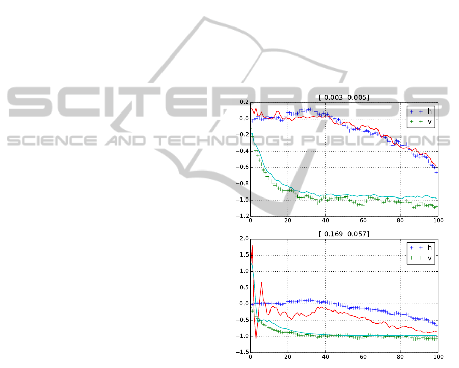
Figures 3, 4 and 5 depict the difference between
the no-cooperation, cooperation and cooperation with
stochastic selection for the nodes i = 0 with the least
observation noise and i = 9 with the highest. The
figures also show the nodes’ MSEs of both esti-
mates. Apparently, under cooperation, node 0 has
very slightly worse MSE connected with the first state
variable, and very slight or no improvement in the
second variable. With respect to the MSEs’ order
10
−3
, the change in this node, best in terms of obser-
vation noise variance, is negligible. On the other side,
the filtration in the “worst” node 9 is significantly bet-
ter.
5 CONCLUSION
The contribution presented the Bayesian approach to
cooperative Kalman filtering in distributed networks,
where the node collaborate in terms of sharing their
measurements. Besides the derivation of the basic co-
operative Kalman filter, a scheme for stochastic se-
lection of adjacent nodes was discussed. It provides
a reasonable way towards decreasing the communi-
cation and computational burden, while retaining the
ability to adapt to evolving statistical properties of
neighbors measurements.
Although the theory was developed under quite re-
strictive assumptions (common model, invariant tran-
sition matrices), their releasing is very simple: it can
be achieved by assuming time-variability and hetero-
geneity in the derivation of the basic Kalman filter in
Section 2.
ACKNOWLEDGEMENT
This work is supported by the Czech Science Founda-
tion, grant no. 14–06678P.
APPENDIX
Lemma 1 (Sherman-Morrison-Woodburry). Let
A, B, C and D be matrices of appropriate dimensions.
Then the following equality holds:
(A + BCD)
−1
= A
−1
B(C
−1
+ DA
−1
B)
−1
DA
−1
.
The (well-known) proof can be found, e.g., in (Meyer,
2000).
Figure 3: Filtering without cooperation: nodes i = 0 and
i = 9 (with least and maximum measurement noises). The
numbers indicate MSEs. Solid line depicts estimates, ’+’
true noisy values.
CollaborativeKalmanFiltration-BayesianPerspective
473
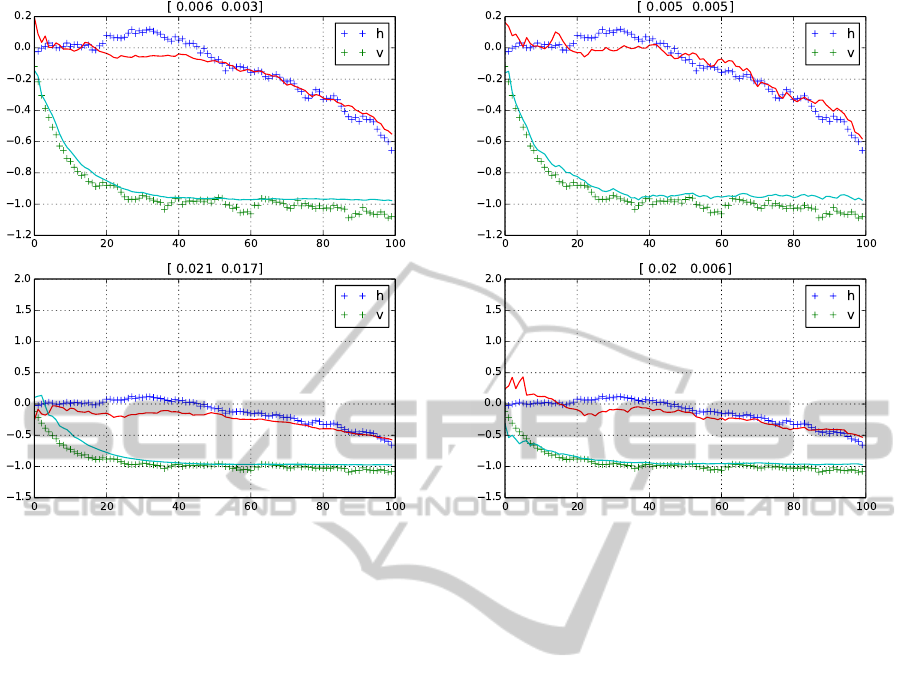
Figure 4: Filtering with cooperation: The same two nodes.
REFERENCES
Cattivelli, F. S., Lopes, C. G., and Sayed, A. H. (2008).
Diffusion Recursive Least-Squares for Distributed Es-
timation over Adaptive Networks. IEEE Trans. Signal
Processing, 56(5):1865–1877.
Cattivelli, F. S. and Sayed, A. H. (2010). Diffusion Strate-
gies for Distributed Kalman Filtering and Smoothing.
IEEE Trans. Automat. Contr., 55(9):2069–2084.
Cattivelli, F. S. and Sayed, A. H. (2011). Analysis of Spatial
and Incremental LMS Processing for Distributed Esti-
mation. IEEE Trans. Signal Processing, 59(4):1465–
1480.
Dedecius, K. and Se
ˇ
ck
´
arov
´
a, V. (2013). Dynamic Diffu-
sion Estimation in Exponential Family Models. IEEE
Signal Process. Lett., 20(11):1114–1117.
Gupta, V., Chung, T. H., Hassibi, B. and Murray, R. M.
(2006). On a stochastic sensor selection algorithm
with applications in sensor scheduling and sensor cov-
erage. Automatica, 42(2), 251-260.
Mo, Y., Ambrosino, R. and Sinopoli, B. (2011). Sensor
selection strategies for state estimation in energy con-
strained wireless sensor networks. Automatica, 47(7),
1330-1338.
Yang, W., Chen, G., Wang, X. and Shi, L. (2014).
Stochastic sensor activation for distributed state esti-
mation over a sensor network. Automatica [in Press].
doi:10.1016/j.automatica.2014.05.025
Dedecius, K. (2014). Diffusion estimation of state-space
models: Bayesian formulation. Submitted to 2014
Figure 5: Filtering with cooperation and stochastic neigh-
bors selection: The same two nodes.
IEEE Machine Learning for Signal Processing Work-
shop.
Meinhold, R. J. and Singpurwalla, N. D. (1983). Under-
standing the Kalman Filter. The American Statistician,
37(2):123–127.
Meyer, C. (2000). Matrix analysis and applied linear alge-
bra. SIAM.
Olfati-Saber, R. (2007). Distributed Kalman filtering for
sensor networks. In 2007 46th IEEE Conference on
Decision and Control, pages 5492–5498. IEEE.
Peterka, V. (1981). Bayesian approach to system identifi-
cation. In Eykhoff, P., editor, Trends and Progress
in System Identification, pages 239–304. Pergamon
Press, Oxford, U.K.
Ribeiro, A., Giannakis, G., and Roumeliotis, S. (2006).
SOI-KF: Distributed Kalman Filtering With Low-Cost
Communications Using the Sign of Innovations. IEEE
Trans. Signal Processing, 54(12):4782–4795.
Simon, D. (2006). Optimal state estimation: Kalman, H
∞
,
and nonlinear approaches. Wiley.
Speyer, J. L. (1978). Computation and Transmission
Requirements for a Decentralized Linear-Quadratic-
Gaussian Control Problem. IEEE Trans. Autom.
Contr., 24(2):266–269.
ICINCO2014-11thInternationalConferenceonInformaticsinControl,AutomationandRobotics
474
