
Swing-up Control of a Single Inverted Pendulum
on a Cart With Input and Output Constraints
Meta Tum
1
, Giyeong Gyeong
2
, Jae Heon Park
2
, and Young Sam Lee
2
1
Robot Department, Inha University, Incheon, Korea
2
Department of Electrical Engineering, Inha University, Incheon, Korea
Keywords:
Cart Inverted Pendulum, Boundary Value Problem, Nonlinear Feedforward Control, Input and Output
Constraints, Linear Feedback Control.
Abstract:
In this paper we propose a new swing-up strategy for a single inverted pendulum. The proposed method has a
feature that can handle the limitation of the pendulum-rail length and actuator constraints using both feedfor-
ward and feedback control. The feedforward trajectories are generated by solving an optimal control problem
having two-point boundary conditions. The limitation of the rail length and the actuator constraints are taken
into account in the problem formulation. Feedback control is combined with the feedforward control to com-
pensate the deviation between the desired trajectories and actual trajectories. The experimental results of the
proposed strategy show that it has a good swing-up performance while satisfying all the imposed constraints.
1 INTRODUCTION
An inverted pendulum system is one of the most pop-
ular experimental apparatuses used for control educa-
tion. The control challenge of an inverted pendulum
comes from the fact that it is nonlinear, unstable, and
underactuated. Besides being used in linear and non-
linear control education, inverted pendulum systems
are used to verify a designed control system. There
are two different types of inverted pendulum systems.
One consists of two links, only one of which is ac-
tuated (Spong and Block, 1995). The other one is a
pendulum on a cart which moves horizontally (Chung
and Hauser, 1995). Similar to an inverted pendulum
on a cart, a rotary inverted pendulum which is called
Furuta pendulum has an advantage of an unbounded
rail length (Furuta et al., 1992). Since swinging up
a pendulum successfully in short time on a short rail
under some constraints of an actuator are very chal-
lenging, various nonlinear swing-up control methods
have been developed. One of the most popular con-
trol approaches applied to an inverted pendulum sys-
tems is so-called energy-based method which is first
proposed by (Wilklund et al., 1993). Some papers
adopted a Lypunov function approach (
˚
Astr
¨
om and
Furuta, 2000) and (Yang et al., 2009). In their ap-
proaches, the stability is guaranteed irrespectively of
the choice of design parameters, but a maximum cart
displacement can be taken into account only by man-
ually adjusting design parameters. The disadvantages
of their approaches are that the rail length limitation
is not taken into account systematically. As a result,
the cart may collide with the wall. Furthermore, the
swing-up time is obtained only after experiments.
Recently, another approach using a combination
of feedforward and feedback control to solve the
swing-up of an inverted pendulum problem was pro-
posed in (Rubi et al., 2002). (Graichen et al., 2007)
implemented that approach on a double inverted pen-
dulum on a cart. The necessary swing-up maneuver
of the double pendulum on the cart is determined by
solving a two-point boundary value problem (BVP)
for the internal dynamics of the pendulum. The two-
point BVP is solved by providing free parameters in
the desired trajectory without considering the input-
output constraints. The results in (Graichen and Zeitz,
2005b) have been further elaborated in (Graichen and
Zeitz, 2005a) such that it can incorporate input con-
straints directly within a feedforward control design
for a non-linear SISO system. Later on, (Graichen
and Zeitz, 2008) proposed a feedforward control de-
sign for a finite-time transition problem of nonlinear
system input-output constraints. To incorporate con-
straints on outputs and its time derivatives, the input-
output dynamics are replaced by a new system, which
is systematically constructed by means of saturation
functions. Disadvantages of this approach are that the
feedforward control input needs to be pre-assumed to
475
Tum M., Gyeong G., Park J. and Lee Y..
Swing-up Control of a Single Inverted Pendulum on a Cart With Input and Output Constraints.
DOI: 10.5220/0005018604750482
In Proceedings of the 11th International Conference on Informatics in Control, Automation and Robotics (ICINCO-2014), pages 475-482
ISBN: 978-989-758-039-0
Copyright
c
2014 SCITEPRESS (Science and Technology Publications, Lda.)

be of a form and the swing-up time must be prede-
fined. A side-stepping of a single inverted pendulum
is used as an example to illustrate their approach. The
input trajectory to the system is a polynomial function
with free parameters which is just one of the possible
combinations, and the final transition time is prede-
fined.
In this paper we also use the combination of feed-
forward and feedback control approach, but our feed-
forward control optimally generates the input trajec-
tory for swing-up maneuver without assuming the
input trajectory form and predefining the swing-up
time. Moreover, it can handle the input-output con-
straints of the system. A typical feedforward control
input trajectory is the transition within a finite-time
interval between two stationary setpoints, one is at the
downright position and the other one is at the upright
position, which makes the system satisfy the bound-
ary conditions (BCs). Feedback controller is used to
correct the error along the nominal trajectory.
This paper is organized as follows. In Section 2, a
mathematical model is provided and a swing-up prob-
lem is described. In Section 3, we describe bound-
ary conditions of the system, the cost function to be
optimized, and the feedforward control design. The
experiment results, parameter optimization, and feed-
back control design will be presented in Section 4.
Finally in Section 5, we make conclusions.
2 PROBLEM STATEMENT
x
θ
l
m
u x
=
&&
cart
center of gravity
pendulum
rail
c
0
x
=
lim
x
side wall side wall
Figure 1: The conceptual diagram of a cart pendulum sys-
tem.
Figure 1 shows the conceptual diagram of a cart pen-
dulum system. A cart pendulum system consists of a
pendulum and a cart that moves along the rail. The
two main outputs are the angle of the pendulum and
the position of the cart. The pendulum is swung by
the cart and the cart is usually driven by an electric
Table 1: Model parameters of the system.
Parameters values
m 0.41 Kg
l 0.22 m
I 0.116 Nms
2
c 0.005 Nms
2
motor. Applying Lagrange’s formulation, one can get
the following differential equation which governs the
movement of the pendulum system:
(I + ml
2
)
¨
θ + ml(cosθ) ¨x = mgl(sin θ) − c
˙
θ (1)
where I is the moment of inertia of a pendulum with
respect to the center of gravity, l the length of the pen-
dulum from the pivot to the center of gravity, m the
mass of the pendulum, g the acceleration of gravity, c
the rotational damping coefficient, θ the angular dis-
placement of the pendulum, x the displacement of the
cart from the center of the rail to any positions on the
rail. Equation (1) shows that the motion of the pen-
dulum is directly governed by the cart acceleration. If
we assume that the acceleration ¨x of the cart serves as
an input u to the system, then the overall model of the
pendulum can be described as follows:
¨x = u (2)
¨
θ =
mgl(sin θ) − c
˙
θ
I + ml
2
−
ml(cos θ)
I + ml
2
u (3)
It is noted that the system described by equation
(2) and (3) is of 4th order. In this paper, we use a lab-
built inverted pendulum system shown in Figure 2 for
the verification of the proposed results. The model
parameters of our lab-built system are given in Table
1. The cart movement is subject to the constraints due
to the limited rail length and the physical limits of a
DC motor used for actuation as follows:
|x| ≤ 0.3m, | ˙x | ≤ 1.3m/s, | ¨x| ≤ 22m/s
2
(4)
Figure 2: A lab-built cart inverted pendulum system used
for experiments.
The purpose of this paper is to develop a swing-
up control method for a cart inverted pendulum that
satisfies the constraints given in equation (4) by ex-
tending the idea presented in (Graichen et al., 2007)
through the optimal control.
ICINCO2014-11thInternationalConferenceonInformaticsinControl,AutomationandRobotics
476

The approach presented in (Graichen et al., 2007)
for the swing-up of a double-pendulum within a finite
time interval t ∈ [0,T ] generates feedforward trajec-
tories for the cart acceleration to steer the pendulum
from the initial downward equilibrium to the termi-
nal upward equilibrium by solving a two-point BVP.
Then the cart is controlled such that it follows the pre-
computed feedforward trajectory and this will erect
the double pendulum. For the robust control perfor-
mance, the authors combine the feedback control to-
gether with feedforward control. However, this ap-
proach has several things to be improved. Firstly, it
confines the feedforward trajectory to be of some pre-
assumed form. Secondly, input and output constraints
are not systematically taken into account. Finally, it
does not use any optimality criterion for the genera-
tion of the feedforward trajectory.
In this paper, we borrow the idea of using feed-
forward control to swing up the pendulum from
(Graichen et al., 2007). However, we extend the re-
sults through the optimal control so that the three lim-
itations mentioned above can be removed.
3 OPTIMAL FEEDFORWARD
CONTROL
The main purpose of the feedforward control is to
generate the input control which makes the cart move
such that the pendulum swings up from the down-
right to the upright position. It is noted that the cart
tracking performance must be good so that the cart
can follow the pre-computed trajectory well. The PD
controller is used as a position controller in the exper-
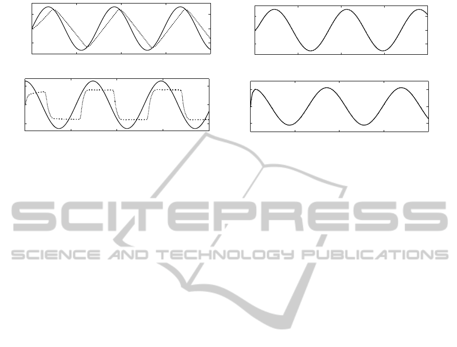
iment. Figure 3 shows the experimental results of the
PD position controller for two sinusoidal references
with different frequencies. It is clearly shown in (a) of
Figure 3 that the cart velocity is limited to 1.55m/s.
When the feedforward control input acceleration re-
quires the cart to move faster than 1.55m/s, the cart
cannot follow the trajectory well. If the required cart
velocity is within constraint, a PD controller can make
the cart follow the desired trajectory well as shown in
(b) of Figure 3. The actual constraints of the system is
shown in equation (5) but in the feedforward control
input generation process, we set the values of the con-
straints smaller than the actual ones which is shown
in equation (4) because we want less error in position
control and to prevent a cart from colliding with the
wall of the pendulum rail.
|x| ≤ 0.4m, | ˙x| ≤ 1.55m/s, | ¨x| ≤ 40m/s
2
(5)
3.1 Feedforward Control Input
Generation
The maneuver of the cart acceleration within a finite-
time interval t ∈ [0,T ] is required to make the system
meet the BCs (6) and (7). The BCs of the system
are the conditions of the position and the velocity of
the cart and the pendulum at downward and upward
equilibrium. The displacement of the cart x(t) and
other states ˙x(t), θ(t), and
˙
θ(t) can be obtained by
solving the differential equation (2) and (3).
x(0) = 0, ˙x(0) = 0, θ(0) = −π,
˙
θ(0) = 0 (6)
x(T ) = 0, ˙x(T ) = 0, θ(T ) = 0,
˙
θ(T ) = 0 (7)
u(0) = 0, u(T ) = 0 (8)
We are interested in starting with zero acceleration
and in forcing it to zero at the final transition time
because, in our lab-built pendulum system, the cart
driven by a DC motor is always accelerated from zero
to any value within constraint, and it will help to re-
duce the bump of the error when we switch from non-
linear swing-up controller to linear controller at the
final transition time. Suppose that the desired control
input acceleration is
u
∗
(t) = ¨x
∗
(t) (9)
which makes the pendulum swing up successfully.
The input acceleration u
∗
(t) makes the cart move
x
∗
(t) within limited rail length with velocity ˙x
∗
(t)
which is within the physical constraint of the cart ac-
tuator. θ
∗
(t) and
˙
θ
∗
(t) are the angle and the angu-
lar velocity of the pendulum respectively which result
from the feedforward control input acceleration u
∗
(t).
Let’s represent the dynamic equation (2) and (3) into
a state space form as follows:
˙
ξ
1
= ξ
2
(10)
˙
ξ
2
= u (11)
˙
ξ
3
= ξ
4
(12)
˙
ξ
4
=
mgl(sin ξ
1
) − cξ
2
I + ml
2
−
ml(cos ξ
1
)
I + ml
2
u (13)
where
ξ
1
= x, ξ
2
= ˙x, ξ
3
= θ, ξ
4
=
˙
θ. (14)
The strategy in generating the feedforward control in-
put presented in (Graichen et al., 2007) is to construct
the control input such that it makes the system meet
the BCs by solving a two-point BVP without includ-
ing the constraints of the system and optimality. In
(Graichen and Zeitz, 2008), the designed feedforward
Swing-upControlofaSingleInvertedPendulumonaCartWithInputandOutputConstraints
477
0 0.5 1 1.5 2
−0.2
0
0.2
time [s]
x[m ]
0 1 2 3 4
−0.2
0
0.2
time [s]
x[m ]
0 0.5 1 1.5 2
−2
0
2
time [s]
˙x[m/s]
0 1 2 3 4
−1
0
1
time [s]
˙x[m/s]
(a) (b)
Figure 3: Tracking performances of a PD position controller for different references: reference(solid) and actual measure-
ment(dotted).
control can deal with input-output constraints by in-
corporating the constraints with pre-assumed input-
output form. The pre-assumed form is provided with
n free parameters if the systems has 2n BCs, and the
transition time is predefined. Due to these disadvan-
tages, the approach cannot generate a feedforward
control trajectory in a flexible form. Furthermore, it
does not use any optimality criterion. In this paper,
the feedforward control input is generated by solving
the following optimal control problem:
Minimize J(ξ,u,t
f
)
subject to constraint (4),
dynamic equations (10),(11),(12), (13),
and boundary conditions (6),(7), (8).
In this paper, we choose to optimize both energy con-
sumption and the cart displacement by taking the cost
function as follows:
J =
∫
T
0
(aξ
2
1
+ bu
2
)d t (15)
where a + b = 1, a, b ∈ R
+
. The parameters a and b
are used to weigh the importance in the optimization.
If a is bigger than b, the optimization will focus on
the cart displacement more than the cart acceleration
and vice versa.
We solve the above nonlinear optimal control
problem with boundary conditions using a newly de-
veloped solver known as GPOPS-II (Patterson and
Rao, 2014).
Remark 1. We can minimize the transition time by
taking the cost function as follows:
J =
∫
T
0
1d t.
3.2 Feedforward Control Input
Trajectories
GPOPS-II solver yields a large variation in the re-
sulting control input trajectories depending on the
cost function to be minimized and the value of con-
straint in (4). A swing-up of an inverted pendulum
in short time with the short displacement of the cart
are very challenging. Therefore, there are many pos-
sible cost functions which may be used in the opti-
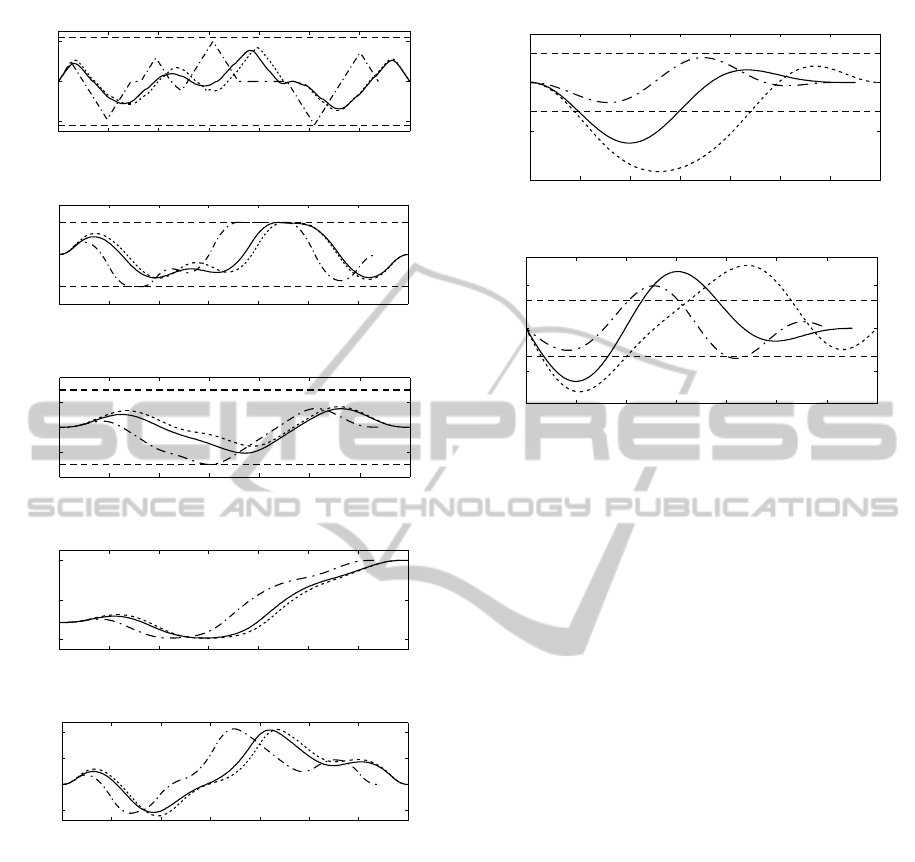
mization for various purposes. Figure 4 shows the
feedforward control and state trajectories for differ-
ent cost functions. The swing-up time is reduced
to 1.3s when the swing-up time is the objective in
the optimization (dash-dotted lines). The swing-up
time is T = 1.4s when we optimize the cart displace-
ment (dotted lines). It shows that when we want the
swing-up time to be as short as possible, the cart ve-
locity goes up to the boundary of constraint, and the
cart displacement is longer than that of other cost
functions. Moreover, the control input acceleration
is much faster than other control input acceleration.
When the cart displacement is optimized, the feedfor-
ward control generated the shortest cart displacement
trajectory. Using a cost function (15) yields a differ-
ent input acceleration and a swing-up motion (solid
lines). Remarkably, the swing-up time was not pre-
defined in the generation of feedforward trajectories,
and all the output states remain within the constraints
of the system.
To clearly show the difference from the approach
presented in (Graichen et al., 2007), we gener-
ated feedforward trajectories using the method given
therein. Figure 5 shows the obtained feedforward
trajectories for the displacement and the velocity of
the cart. Trajectories were generated for the three
ICINCO2014-11thInternationalConferenceonInformaticsinControl,AutomationandRobotics
478
0 0.2 0.4 0.6 0.8 1 1.2 1.4
−20
0
20
time [s]
¨x
∗
£
m/s
2
¤
cart acceleration trajectories
0 0.2 0.4 0.6 0.8 1 1.2 1.4
−2
0
2
time [s]
˙x
∗
[m/s]
cart velocity trajectories
0 0.2 0.4 0.6 0.8 1 1.2 1.4
−0.4
−0.2
0
0.2
time [s]
x
∗
[m]
cart position trajectories
0 0.2 0.4 0.6 0.8 1 1.2 1.4
−4
−2
0
time [s]
θ
∗
[rad]
angle trajectories
0 0.2 0.4 0.6 0.8 1 1.2 1.4
−5
0
5
10
time [s]
˙
θ
∗
[rad/s]
angular velocity trajectories
Figure 4: The possible feedforward trajectories for swing-
up maneuver of the inverted pendulum system for different
cost functions.
swing-up times, which are T = 1.2(dash-dot), T =
1.3(solid), and T = 1.4(dotted). It is shown that the
trajectories generated for the swing-up time T = 1.3
and T = 1.4 satisfy neither the displacement con-
straint nor the velocity constraint. Trajectories for
T = 1.2 satisfy the displacement constraint. How-
ever, they go beyond the velocity constraint. Vio-
lation of the cart displacement constraint will result
in the cart’s collision with the wall during swing-up.
Furthermore, dissatisfaction of the velocity constraint
means that the swing-up control is not possible using
the given actuator, which also means that we have to
replace the actuator with better ones for the swing-up.
0 0.2 0.4 0.6 0.8 1 1.2 1.4
−1
−0.5
0
0.5
time [s]
x
∗
[m]
cart position trajectories
0 0.2 0.4 0.6 0.8 1 1.2 1.4
−2
0
2
time [s]
˙x
∗
[m/s]
cart velocity trajectories
Figure 5: Feedforward trajectories generated by the method
of (Graichen et al., 2007) for different values of T : T =
1.2(dash-dot), T = 1.3(solid), T = 1.4(dotted).
Since the trajectories generated by the proposed
approach consider the given constraints systemati-
cally, we can make the most of the performance of the
actuator and protect the system from collision. This
will give much better freedom in choosing the actua-
tor for the system.
4 EXPERIMENTAL RESULTS
Swing-up maneuver is experimentally realized with a
lab-built pendulum shown in Figure 2. Two incremen-
tal encoders with the resolution of 5000 pulses/rev are
used, one for measuring the displacement of the cart
and the other one for measuring the angular displace-
ment of pendulum. All the measurement information
is transmitted to a controller board with a sample time
of 1 ms. The nominal trajectories θ
∗
(t),
˙
θ
∗
(t), x
∗
(t),
and feedforward control acceleration u
∗
(t) = ¨x
∗
, t ∈
[0,T ] are stored in lookup tables. We use a PD po-
sition controller to generate the required acceleration
u
∗
(t) by tracking the position reference x
∗
(t), which is
obtained by double integration of u
∗
(t). Coefficients
for the PD controller are chosen to be K
p
= 700 and
K
d
= 20.
4.1 Model Parameter Estimation
Using only nonlinear feedforward control to swing
up the pendulum is hard to succeed because the un-
certainty of the model parameters yields the infeasi-
Swing-upControlofaSingleInvertedPendulumonaCartWithInputandOutputConstraints
479
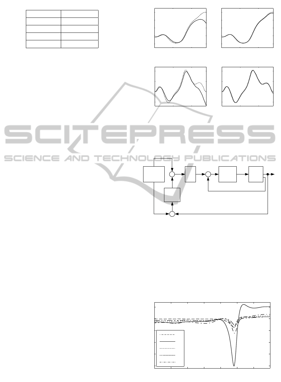
Table 2: Estimated model parameters of the system.
Parameters values
m 0.4 Kg
l 0.24 m
I 0.016 Nms
2
c 0.005 Nms
2
ble feedforward trajectories. The external disturbance
and the poor cart tracking performance are also the
factors which make the control unsuccessful in real
experiments. If the feedforward has a big error, the
feedback controller cannot correct the error properly.
Therefore the accurate feedforward control is neces-
sary. (a) of Figure 6 shows the experimental results
of the angle and the angular velocity of the pendulum
in open loop corresponding to the model parameters
given in Table 1. The simulation and experiment re-
sult are much different. This is because model param-
eter values used in the simulation and the actual ones
of the real system are different. To enhance the accu-
racy of the model parameter values, the optimization-
based adjustment is needed to find a set of correct val-
ues of model parameters by minimizing the following
cost function:
J =
∫
T
0
(θ
∗
(t) − θ(t))
2
+ (
˙
θ
∗
(t) −
˙
θ(t))
2
d t (16)
where θ
∗
(t) and
˙
θ
∗
(t) are simulation trajectories
which are generated by using the model parameter
values in Table 1. θ(t) and
˙
θ(t) are the actual mea-
sured angle and angular velocity respectively in the
open loop experiment. We use ‘fmincon’, the opti-
mization function provided in Matlab toolbox to solve
the optimization problem. We regenerated feedfor-
ward trajectories after getting a new set of the model
parameters. It is noted that the new set of model pa-
rameters are not the actual values of the real system.
Instead, it is just a possible combination that verifies
the dynamic equation (1). The new set of model pa-
rameters are shown in Table 2. (b) of Figure 6 is the
experimental results of new model parameters.
4.2 Linear Feedback Controller
The nonlinearity and instability in dynamics make
the pendulum sensitive to the perturbation which is
caused by the external disturbance and the delay in
the system. As a result, the pendulum may not fol-
low the nominal trajectory. The realization of the
swing-up of an inverted pendulum requires a feedback
controller to correct the derivation between the ac-
tual states (x, ˙x,θ,
˙
θ) and desired states (x
∗
, ˙x
∗
,θ
∗
,
˙
θ
∗
).
Figure 7 is a two-degree-of-freedom control scheme
0 0.5 1
−4
−3
−2
−1
0
time [s]
θ
∗
[rad]
angle
0 0.5 1
−4
−3
−2
−1
0
time [s]
θ
∗
[rad]
angle
0 0.5 1
−5
0
5
10
time [s]
˙
θ
∗
[rad/s]
angular velocity
0 0.5 1
−5
0
5
10
time [s]
˙
θ
∗
[rad/s]
angular velocity
(a) (b)
Figure 6: The open-loop experimental results for the angle
and the angular velocity using (a) default parameters and
(b) the estimated parameters.
voltage
FB
control
PD
position
controller
System
FF
trajectories
*
ξ
+
−
∆
u
+
+
u
d
x
+
−
x
e
ξ
*
u
∫∫
ξ
∆
Figure 7: The 2-DOF control scheme for the swing-up.
of feedforward and feedback control. In order to com-
pensate the possible steady state error in the cart posi-
tion, the inverted pendulum model is dynamically ex-
tended by the disturbance model
˙
˜x = x as in (Graichen
et al., 2007). The new desired system becomes
˙
ξ
∗
= f (ξ
∗
,u
∗
) (17)
where
ξ
∗
= [x
∗
, ˙x
∗
, θ
∗
,
˙
θ
∗
, ˜x
∗
] (18)
0 0.2 0.4 0.6 0.8 1 1.2 1.4
−200
−150
−100
−50
0
50
time [s]
feedback gain
k1
k2
k3
k4
k5
Figure 8: Time-varying LQ feedback gain.
ICINCO2014-11thInternationalConferenceonInformaticsinControl,AutomationandRobotics
480
and
˜x
∗
(t) =
∫
t
0
x
∗
(τ)dτ. (19)
We design feedback control for nonlinear system
based on linear system theory as in (Graichen et al.,
2007). This leads to linear time-varying system and
the system is linearized as follow:
∆
˙
ξ = A(t)∆ξ + B(t)∆u (20)
where
A(t) =
∂ f
∂ξ
ξ
∗
(t),u
∗
(t)
, (21)
B(t) =
∂ f
∂u
ξ
∗
(t),u
∗
(t)
(22)
where k(t) is the time varying feedback gain, ξ
∗
is the
desired state trajectories, and u
∗
is the desired control
trajectory. Time-varying feedback gain k(t) can be
obtained by solving an optimal LQ (linear quadratic)
control which minimize the objective function as fol-
lows:
J =
∫
T
0
(∆ξ
T
Q∆ξ + ∆u
T
R∆u)dt
+∆ξ
T
(T )S∆ξ(T) (23)
where Q and S ∈ R
5×5
are the symmetric positive
semi-definite matrices and R is a positive scalar. Feed-
back gain k(t), t ∈ [0,T ] is determined by
k(t) = R
−1
B
T
(t)P(t), (24)
where P(t) is the solution on [0,T ] of the matrix Ric-
cati differential equation (RDE) as follows:
˙
P = PB(t)R
−1
B
T
(t)P − PA(t) − A
T
(t)P − Q. (25)
It is noted that P(T ) = S, where S is determined
by solving the algebraic Riccati equation (25) with
˙
P = 0. The weighting matrix Q is chosen to be the
diagonal matrix (800,3000,0,0, 100) and the R = 50.
Figure 8 shows the time-varying feedback gain
k
i
(t), i = 1,·· · ,5 in the time interval t ∈ [0, T ]. In
the time interval t ∈ [0.8,1] the feedback gain has a
big oscillation because in that time interval, the pen-
dulum is about to lie down on the horizontal axis and
its controllability is very weak and lose its controlla-
bility when the pendulum is at the 90 degree position.
4.3 Experimental Results of Combined
Control
We performed two control experiments. One used
only generated control input trajectory, which is ac-
tually called open-loop control. The other one used
the combination of feedforward and feedback control
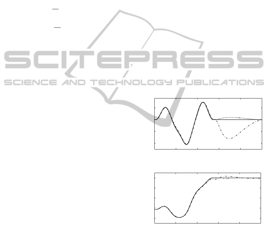
as shown in the control scheme in Figure 7. Fig-
ure 9 shows the experimental results of the cart dis-
placement x(t) and angular displacement θ(t). The
open-loop control gives a good performance only at
the beginning. The pendulum tracked smoothly along
the nominal trajectory almost up to the upright po-
sition. When we switch from the swing-up control
to the stabilizing linear controller at the upright posi-
tion, the stabilizing linear controller could handle the
small error and steer the pendulum to the upright po-
sition. However, relatively big bump is encountered
after switching. The dash-dot line in the Figure 9 de-
notes the open-loop experiment results. The dotted
line represents a tracking performance of pendulum
when we performed the closed-loop control. It shows
the effectiveness of feedback controller which com-
pensates the deviation between the actual states and
the desired states. As a result, the pendulum tracked
the nominal trajectory well up to the upright position
and then smoothly switched from the nonlinear con-
troller to the linear controller.
0 0.5 1 1.5 2 2.5
−0.2
−0.1
0
0.1
time [s]
x[m ]
cart position
0 0.5 1 1.5 2 2.5
−4
−3
−2
−1
0
time [s]
θ[rad]
angle
Figure 9: Comparison of the experimental results: open
loop trajectory(dash-dot), closed loop trajectory(dotted),
desired trajectory(solid).
5 CONCLUSIONS
The presented approach in this paper extends the pre-
vious results such that it can handle the rail length
Swing-upControlofaSingleInvertedPendulumonaCartWithInputandOutputConstraints
481

limitation and actuator constraints systematically. In
this approach, the swing-up maneuver of an inverted
pendulum from downward equilibrium to upward
equilibrium is accomplished within a two-degrees of
freedom control scheme consisting of nonlinear opti-
mal feedforward controller and the optimal feedback
controller. The feedforward control input trajectory
is generated by the newly developed optimal control
solver that can handle the input and output constraints
of the system. Simulation and experimental results
showed close resemblance, which shows that the pro-
posed method is quite practical. The swing-up of
the inverted pendulum through the proposed method
turned out to be always successful. The proposed ap-
proach enables one to make the most of performance
of the given actuator. The presented approach can be
extended to the swing-up control of a double or triple
inverted pendulum without much of modification.
ACKNOWLEDGEMENTS
This research was supported by the MSIP(Ministry
of Science, ICT and Future Planning), Korea, un-
der the C-ITRC(Convergence Information Technol-
ogy Research Center)support program(NIPA-2014-
H0401-14-1003) supervised by the NIPA(National IT
Industry Promotion Agency) and was also supported
by Korea Electric Power Corporation Research Insti-
tute through Korea Electrical Engineering & Science
Research Institute (grant number: R13GA04).
REFERENCES
˚
Astr
¨
om, K. and Furuta, K. (2000). Swinging up a pendulum
by energy control. Automatica, 36(2):287–295.
Chung, C. C. and Hauser, J. (1995). Nonlinear control of a
swinging pendulum. Automatica, 31(6):851–862.
Furuta, K., Yamakitan, M., and Kobayashi, S. (1992).
Swing-up control of inverted pendulum using pseudo-
state feedback. Journal of Systems and Control Engi-
neering, 206:263–269.
Graichen, K., Treuer, M., and Zeitz, M. (2007). Swing up
of the double pendulum on a cart by feedforward and
feedback control with experimental validation. Auto-
matica, 43:63–71.
Graichen, K. and Zeitz, M. (2005a). Feedforward control
design for nonlinear systems under input constraints.
In Meuer, T., Graichen, K., and Gilles, E. D., edi-
tors, Control and observer design for nonlinear finite
and infinite dimensional systems, LNCIS Volumn 322,
pages 235–252. Springer.
Graichen, K. and Zeitz, M. (2005b). Nonlinear feedfoward
and feedback tracking control with input constraints
solving the pendubot swing-up problem. In Proceed-
ings of the 16th IFAC World Congress, pages 841–841,
Prague, Czech.
Graichen, K. and Zeitz, M. (2008). Feedforward control
design for finite-time transition problems of nonlin-
ear systems with input and output constraints. IEEE
Transactions on Automatic Control, 53(5):1273–
1286.
Patterson, M. A. and Rao, A. V. (2014). GPOPS - II Version
1.0: A general-purpose Matlab toolbox for solving op-
timal control problems using variable-order Gaussian
quadrature collocation methods.
Rubi, J., Rubio, A., and Avello, A. (2002). Swing-up con-
trol problem for a self-erecting double inverted pen-
dulum. IEE Proceedings-Control Theory and Appli-
cations, 149(2):169–175.
Spong, M. and Block, D. (1995). The pendubot: a mecha-
tronic system for control research and education. In
Proceedings of the 35th IEEE Conference on Decision
and control,, pages 555–556, New Orleans, USA.
Wilklund, M., Kristenson, A., and
˚
Astr
¨
om, K. (1993). A
new strategy for swing up an inverted pendulum. In
Proceedings of IFAC 12th world congress, volume 9,
pages 151–154, Sydney, Australia.
Yang, J. H., Shim, S. Y., Seo, J. H., and Lee, Y. S. (2009).
Swing up control for an inverted pendulum with re-
stricted cart rail length. International Journal of Con-
trol, Automation, and Systems, 70(4):674–680.
ICINCO2014-11thInternationalConferenceonInformaticsinControl,AutomationandRobotics
482
