
Observer-based controller Design for Remotely Operated Vehicle ROV
Adel Khadhraoui
1
, Lotfi Beji
1
, Samir Otmane
1
and Azgal Abichou
2
1
University of Evry, IBISC Laboratory, EA 4526, 40 rue du Pelvoux, 91020 Evry, France
2
Polytechnic School of Tunisia, LIM Laboratory, BP743, 2078 La Marsa, Tunisia
Keywords:
Observer, Controller, Estimation, Lyapunov theory, Stabilization, ROV.
Abstract:
This paper presents a method to design an observer-based controller that simultaneously solves global esti-
mation of state and asymptotic stabilization of an underactuated remotely operated vehicle moving in the in
three-dimensional. The vehicle does not have a sway and roll actuator and has only position and orienta-
tion measurements available. The control development is based on Lyapunov’s direct method for nonlinear
system.
1 INTRODUCTION
In many works on the control of dynamical systems,
the state vector is assumed to be measured. However,
on a practical level, this assumption is not always
true. Indeed, for technical or economical reasons, it
is difficult or impossible to measure all the state vari-
ables of the system. Hence, the need to fully know
the state variables of the system is often a necessity
in the phases of modeling and identification, diagno-
sis and control systems. All these problems require
knowledge of the state vector, not accessible to mea-
surement data, which makes the design of an observer
a primordial task in control theory.
The problem of observation has been studied by
a number of researchers these last years The linear
case has been solved by Kalman and Luenberger, but
the nonlinear case is still an active domain of re-
search. The high-gain observer approach which is
closely related to triangular structure has been devel-
oped by (Gauthier et al., 1992),(Gauthier and Kupka,
1994) and is derived from the uniform observabil-
ity of nonlinear systems. Other methods have been
developed: Kazantzis and Karavaris (Kazantzis and
Kravaris, 1997), the backstepping observer which
uses the Lyapunov auxiliary theorem and a direct co-
ordinate transformation in design in (Li and Qian,
2006) and (Arcak, 2002). Switching or multi-model
observers based on Linear Matrix Inequality tech-
niques are used for the observation of LPV, quasi-
LPV or Takagi-Sugeno fuzzy systems (Takagi and
Sugenou, 1985), (Dounia et al., 2012), (Chang and
Chen, 2013). The adaptive observer was proposed in
(Pourgholi and Majd, 2012), parameter and state es-
timation problem in the presence of the perturbation.
In (F. Rezazadegan and Chatraei, 2013), an adapta-
tive control law for 6 DOF model is drived for the tra-
jectory tracking problem of underactuated underwater
vehicle in the presence of parametric uncertainty. The
famous Kalman filter algorithm, which assumes white
and Gaussian disturbances and noises has been suc-
cessfully applied to the estimation of state variables
of nonlinear system in numerous engineering appli-
cations. Applications such as State and parameter
estimation of aircraft and Unmanned Aerial Vehicles
(UAV’s) (Langelaan, 2006), (Rigatos, 2012), are all
examples of aerospace applications for the Kalman
filter. In (Berghuis and Nijmeijer, 1993) the authors
propose a nonlinear observer-based controller strat-
egy for robot manipulators based on passivity theory.
The controller and observer are designed to use the
structure of each other and semi-global exponential
stability of the observer error and controller error dy-
namics are proven. In (Shen et al., 2011), (Li et al.,
2011), (Li et al., 2013), the problem of finite-time
observers has been considered and global finite-time
observer are designed for nonlinear system which
are uniformly observable and globally Lipschitz. In
(Fridman et al., 2008), a higher-order sliding-mode
observer is proposed to estimate exactly the observ-
able states and asymptotically the unobservable ones
in multi-input-multi-outputnonlinear system with un-
known inputs and stable internal dynamics. In this
paper, we propose to control Remotely Operated Ve-
hicles (ROV’s) for exploration in sub-sea historical
sites. The main contribution in this paper is to design
200
Khadhraoui A., Beji L., Otmane S. and Abichou A..
Observer-based controller Design for Remotely Operated Vehicle ROV.
DOI: 10.5220/0005019102000207
In Proceedings of the 11th International Conference on Informatics in Control, Automation and Robotics (ICINCO-2014), pages 200-207
ISBN: 978-989-758-039-0
Copyright
c
2014 SCITEPRESS (Science and Technology Publications, Lda.)

a nonlinear observer to estimate the linear and angu-
lar velocity of the ROV. The remainder of this paper
is organized as following. In Section 2 the kinematic
and dynamic model of the ROV are presented. The
design observer for estimating the linear and angu-
lar velocity in the presence of constants disturbance
is synthesized in Section 3. In Section 4 a feedback
law is proposed to stabilize the system of the ROV at
the origin. The theoretical results are illustrated by
simulations in section 5.
2 ROV MODEL DESCRIPTION
The ROV has a close frame structure and is equipped
with two cameras which allow us the Tele-exploration
in mixed-reality sites (see Figure 1). This vehicle is
actuated with two reversible horizontal thrusters F
1x
and F
2x
for surge and yaw motion, and a reversible
vertical thruster F
3z
for heave motion. A 150 meters
cable provides electric power to the thrusters and en-
ables communication between the vehicle sensors and
the surface equipment (see Figure 1).
2.1 Coordinate Frame
Underwater vehicle models are conventionally repre-
sented by a six degrees of freedom nonlinear set of
first order differential equations of motion. Two ref-
erence frames are used to describe the vehicles states,
R
0
for inertial frame, and R
v
for local body-fixed
frame with its origin coincident with the vehicles cen-
ter of buoyancy, and the 3 principle axes in the vehi-
cles surge, sway and heave directions (see Figure 1).
Figure 1: Body-fixed frame and earth-fixed frame for ROV.
2.2 ROV Equations of Motion
The mathematical model of a ROV in 6 DOF can be
described by:
˙
η
1
= J
1
(η
2
)ν
1
,
˙
η
2
= J
2
(η
2
)ν
2
M
˙
ν = −C(ν)ν− D(ν)ν− g(η) + τ
(1)
where η = [η
1
η
2
]
T
with η
1
= [x y z]
T
and η
2
=
[φ θ ψ]
T
is the position and orientation vector in earth-
fixed frame, ν = [ν
1
ν
2
]
T
with ν
1
= [u v w]
T
and
ν
2
= [p q r]
T
is the velocity and angular rate vec-
tor in body-fixed frame, the symmetric positive def-
inite inertia matrix M = M
v
+ M
a
includes the iner-
tia M
v
of the vehicle as a rigid body and the added
inertia M
a
due to the acceleration of the wave, the
skew symmetrical matrix C(ν) is the matrix of Cori-
olis and centripetal, the hydrodynamic damping term
D(ν) = D
L
+ D
Q
(ν) (positive definite diagonal ma-
trix) takes into account the dissipation of energy due
to the friction exerted by the fluid surrounding AUV,
where D
Q
(ν) and D
L
are the quadratic and linear drag
matrices, respectively. The terms g(η) is the restor-
ing force vector, τ is the input torque vector, and the
transformation matrices J
1
(η
2
) and J
2
(η
2
) are as fol-
lowing:
J
1
(η
2
) =
cθcψ sθsφcψ−sψcφ sθcφcψ+ sψsφ
cθsψ sθsφsψ+ cψcφ sθcφsψ− cψsφ
−sθ cθsφ cθcφ
!
J
2
(η
2
) =
1 sφtθ cφtθ
0 cφ −sφ
0
sφ
cθ
cφ
cθ
J(η
2
) =
J
1
(η
2
) 0
0 J
2
(η
2
)
where c(.) = cos(.), s(.) = sin(.), t(.) = tan(.).
Remark 2.1. For the sake of simplicity, external dis-
turbances such as ocean current are not taken into
consideration. The detailed definition of each element
in (1) and the influence of external environment can be
found in (Fossen, 1994). For the ROV one excludes an
attitude in pitch equal to
π
2
.
Assumption 2.2. 1) ROV has an (xz) and (yz) two
planes of symmetry, surge is decoupled from pitch
modes.
2) The center of gravity is vertically aligned with the
center of buoyancy, i.e.,[0, 0, −z
g
]
T
.
The autonomous underwater vehicle (ROV) is a
complex nonlinear system described by twelve state
variables and three controls. The full model can be
found in (Khadhraoui et al., 2013). The kino-dynamic
model of the ROV in low speed can be written in the
form presented below:
˙
η
1
= J
1
(η
2
)ν
1
,
˙
η
2
= J
2
(η
2
)ν
2
M
˙
ν = −D
L
ν− g(η) + τ
(2)
Thus, the general mathematical model of the ROV in
surge, sway, heave and heading motion is given by:
Observer-basedcontrollerDesignforRemotelyOperatedVehicleROV
201

˙u =
m
55
m
11
m
55
−m
2
15
[d
u
u+ (F
W
− F
B
))sθ+τ
u
]
−
1
m
22
[d
q
q+ z
g
F
B
sθ]
˙v =
m
44
m
22
m
44
−m
2
24
[d
v
v+ (F
W
− F
B
)cθsφ]
˙w =
1
m
33
[d
w
w−(F
W
− F
B
)cθcφ+ τ
w
]
˙p =
1
m
44
[d
p
p− z
g
F
B
cθsφ]
˙q =
m
11
m
11
m
55
−m
2
15
[d
q
q+ z
g
F
B
sθ]
−
m
15
m
11
m
55
−m
2
15
[d
u
u+ (F
W
− F
B
))sθ+τ
u
]
˙r =
1
m
66
[d
r
r+ τ
r
]
˙x = cθcψu+ (sθsφcψ− sψcφ)v
+ (sθcφcψ+ sψsφ)w
˙y = cθsψu+ (sθsφsψ+ cψcφ)v
+ (sθcφsψ− cψsφ)w
˙z = −sθu+cθsφv+cθcφw
˙
φ = p+ sφtanθq+cφtanθr
˙
θ = cφq− sφr
˙
ψ =
sφ
cθ
q+
cφ
cθ
r
(3)
where d
u
, d
v
, d
w
, d
p
, d
q
and q
d
are the drag param-
eters of the ROV. The submerged weight F
W
, and the
buoyancy force F
B
, are given by
F
W
= m.g, F
B
= ρ.∇.g
where g is the gravitational constant, ρ is the density
of the fluid and ∇ is the volume of the ROV.
Having accurate ROV-observer motion informa-
tion, namely the position information η
1
, η
2
and
velocity information ν
1
, ν
2
is crucial for the con-
troller to work properly. Unfortunately, among these
parameters only the 3-dimension position informa-
tion η
1
and attitudes information η
2
are available
from the vehicles sensor system and underwater
acoustic positioning system; the velocity could not
be measured directly. Also, the position information
obtained through the measurement is uncertain due
to noise and other imperfections. To handle this
problem, estimation is applied to the measurements.
3 OBSERVER DESIGN
In the sequel, we consider that the measurements are
the position vector η
1
and the orientation vector η
2
,
and our objective is to estimate the linear and angular
velocities from these measurement.
3.1 Nominal Case
Proposition 3.1. Let us consider the system (2).
Then, there exist a diagonal positive definite constant
matrix L
1
(control gain matrix) and a matrix depend-
ing on the state L
2
(η) for which system (2) admits the
following asymptotic observer:
˙
b
η = J(η
2
)
b
ν− L
1
(η−
b
η)
M
˙
b
ν = −D
L
b
ν−g(η) +τ−L
2
(η)(η−
b
η)
(4)
Proof. According to the system dynamics (2) and the
given observer (4), the error dynamics becomes:
˙
e
η = J(η
2
)
e
ν− L
1
e
η
M
˙
e
ν = −D
L
e
ν− L
2
(η)
e
η
(5)
where
e
η = η −
b
η and
e
ν = ν−
b
ν.
We consider the following Lyapunov function:
V
1
=
1
2
(
e
η
T
e
η+
e
ν
T
e
ν)
(6)
The time derivative of V
1
can be expressed as:
˙
V
1
= −
e
η
T
L
1
e
η−
e
ν
T
M
−1
D
L
e
ν+
e
η
T
J(η
2
)
e
ν−
e
ν
T
M
−1
L
2
(η)
e
η
(7)
If we take
L
2
(η) = MJ(η
2
)
Then, equation (7) become
˙
V
1
= −
e
η
T
L
1
e
η−
e
ν
T
M
−1
D
L
e
ν
(8)
then,
˙
V
1
≤ −λ
1
k
e
η k −λ
2
k
e
ν k (9)
where λ
1
and λ
2
are the minimum eigenvalues of L
1
and M
−1
D
L
, respectively.
By using the Lyapunov theory, we conclude that sys-
tem (5) is asymptotically stable. then, the proposed
observer allows us to estimate all the state vector
asymptotically.
3.2 Perturbed Case
In the presence of environmental constants distur-
bances Θ, the dynamics of the ROV can be written
M
˙
ν = −D
L
ν− g(η) + Θ + τ
(10)
and we define the dynamic observer at the forme
M
˙
b
ν = −D
L
b
ν− g(η) +
b
Θ+ τ
(11)
ICINCO2014-11thInternationalConferenceonInformaticsinControl,AutomationandRobotics
202

where Γ is the diagonal positive definite matrix and
b
Θ
is an estimate of Θ verify
˙
b
Θ = Γ
e
ν. We consider the
following Lyapunov function candidate
W
Θ
=
1
2
e
ν
T
M
e
ν+
1
2
e
Θ
T
Γ
−1
e
Θ
(12)
The time derivativeofW
Θ
can be expressed as follows
˙
W
Θ
= −D
L
e
ν
2
(13)
By using La Salle invariance principle (Khalil, 2002),
we conclude that
e
ν is globally asymptotically stable.
Remark 3.2. As the terms
b
Θ contains the vector un-
certainty ν, it is sufficient to replace the expression
e
ν = ν−
b
ν in the expression of
˙
b
Θ
b
Θ(t) =
b
Θ(t
0
) + Γ
Z
t
t
0
(ν−
b
ν)(σ)dσ
like that ν = J
−1
(η
2
)
˙
η, then
b
Θ(t) =
b
Θ(t
0
) + Γ
Z
t
t
0
(J
−1
(η
2
)
˙
η−
b
ν)(σ)dσ
which gives
b
Θ(t) =
b
Θ(t
0
) + Γ
Z
η(t)
η(t
0
)
J
−1
(σ
′
)dσ
′
− Γ
Z
t
t
0
b
ν(σ)dσ
4 OUTPUT-FEEDBACK
OBSERVER
This section describes the design of the control-based
observer. Based on the estimated states, we will try to
stabilize the kino-dynamic model:
˙
η = J(η
2
)ν
M
˙
ν = −D
L
ν− g(η) + τ
˙
e
η = J(η
2
)
e
ν− L
1
e
η
M
˙
e
ν = −D
L
e
ν− L
2
(η)
e
η
(14)
The control laws required for the stabilization task are
given in the following proposition.
Proposition 4.1. Let k
u
, k
w
and k
r
three nonnegative
reel numbers, considered large enough. Then, with
the action of the following feedback laws
τ
u
=
−(m
2
15
−m
11
m
55
)k
u
m
55
[bu+ k
q
bq+ k
x
x+ k
θ
θ]
τ
w
= −m
33
k
w
[ bw+ k
z
z] + ϖ
τ
w
τ
r
= −m
66
k
r
[br+ k
ψ
ψ]
(15)
where ϖ
τ
w
is a constant parameter will be specified
later. k
x
, k
z
, k
θ
, k
ψ
and k
q
are positives constants. The
system (14) is locally asymptotically stable at the ori-
gin.
Proof. For an under-atuated system, the position vec-
tor can be partitioned to actuated and non-actuated
states as
η = [η
a
η
u
]
T
(16)
where, η
a
= [x z θ ψ]
T
is the actuated states of the
ROV and η
u
= [y φ]
T
is the non-actuated states.
Step 1) Stability analysis of actuated state:
The corresponding linearized around zero of the
actuated system is given by:
˙u = −α
1
u+ α
2
q+ α
3
θ+ τ
u
˙x = u
˙w = −γ
1
w+ γ
2
+ τ
w
˙z = w
˙q = β
1
u− β
2
q+ β
3
θ+ βτ
u
˙
θ = q
˙r = −ρr + τ
r
˙
ψ = r
(17)
where α
i
=, β
i
, γ
i
, γ
i
, π
i
and ρ are positive constants
depends on the ROV fixed parameters.
We consider the following Lyapunov function candi-
date
V
2
=
1
2
{x
2
+ (u+ x)
2
+ θ
2
+ (q+ θ)
2
+ z
2
+ (z+ w)
2
+ ψ
2
+ (ψ + r)
2
}
(18)
The time derivative of V
2
can be expressed as:
˙
V
2
= xu+ (x+ u)(u− α
1
u+ α
2
q− α
u
θ+ τ
u
)
+ θq+ (q+ θ)(q− β
1
q+ β
2
+ α
q
θ+ βτ
u
)
+ zw+ (z+ w)(w− γ
1
w− γ
2
+ τ
w
))
+ ψr+ (ψ + r)(r − ρr + τ
r
)
(19)
by using (15) given in the proposition and we take
ϖ
τ
w
= γ
2
, equation (19) becomes:
˙
V
2
= (x+ u)[(1− α
1
)u− k
u
bu+ α
2
q− k
u
k
q
bq]
+ (x+ u)[(α
u
− k
u
k
θ
)θ− k
u
k
x
x] + xu
+ (q+ θ)[(1− β
1
)q− kk
q
bq+ β
2
u− kbu]
+ (q+ θ)[(α
q
− kk
θ
)θ− kk
x
x] + θq
+ (z+ w)[(1− γ
1
)w− k
w
bw− k
w
k
z
z] + zw
+ (ψ+ r)[(1− ρ)r− k
r
br − k
r
k
ψ
ψ] + ψr
(20)
where k = βk
u
. We consider the coordinate:
u = eu+ bu, q = eq+ bq, w = ew+ bw, r = er+ br
The time derivative of V
2
becomes:
Observer-basedcontrollerDesignforRemotelyOperatedVehicleROV
203

˙
V
2
= −k
1
u
2
− k
2
x
2
− k
3
q
2
− k
4
θ
2
− k
5
w
2
− k
6
z
2
− k
7
r
2
− k
8
ψ
2
+ ϖ
1
xu+ϖ
2
θq+ϖ
3
xq+ϖ
4
θu
+ ϖ
5
θx+ ϖ
6
uq+ϖ
7
zw+ϖ
8
ψr+ k
w
(z+w) ew
+ k
r
(ψ+ r)er(x+ u+θ+ q)(k
u
eu+ k
u
k
q
eq)
(21)
where
k
1
= k
u
− 1+α
1
, k
2
= k
u
k
x
, k
3
= kk
q
− 1+β
2
k
4
= kk
θ
, k
5
= k
w
− (1− γ
1
), k
6
= k
w
k
z
k
7
= k
r
− (1− ρ), k
8
= k
r
k
ψ
ϖ
1
= 2− α
1
− k
u
(1+k
x
), ϖ
2
= 2− β
2
− k(k
q
+ k
θ
)
ϖ
3
= β
1
− k
u
(β+k
θ
), ϖ
4
= α
2
− k
u
(k
q
+ βk
x
)
ϖ
5
= β
1
+ α
2
− k
u
(β+k
q
), ϖ
6
= −k
u
(βk
x
+ k
θ
)
ϖ
7
= 2− γ
1
− k
w
(1+k
z
), ϖ
8
= 2− ρ− k
r
(1+k
ψ
)
In the above expression, we remark that the last terms
have uncertain signs. For the analysis we will use the
Young’s inequality (see Appendix C for the details),
with the quantities ε
i
as positive constants, we obtain:
˙
V
2
≤ −(k
1
− ε
1
)u
2
− (k
2
− ε
2
)x
2
− (k
3
− ε
3
)q
2
− (k
4
− ε
4
)θ
2
− (k
5
− ε
5
)w
2
− (k
6
− ε
6
)z
2
− (k
7
− ε
7
)r
2
− (k
8
− ε
8
)ψ
2
+ k
w
(z+w) ew
+ k
r
(ψ+ r)er + (x+ u)(k
u
eu+ k
u
k
q
eq)
+ (θ+q)(keu + kk
q
eq)
(22)
We consider the following Lyapunov function candi-
date
V
3
= V
1
+V
2
(23)
Taking account of (8) and (22), the time derivative of
V
3
can be expressed as:
˙
V
3
≤ −(k
1
− ε
1
)u
2
− (k
2
− ε
2
)x
2
− (k
3
− ε
3
)q
2
− (k
4
− ε
4
)θ
2
− (k
5
− ε
5
)w
2
− (k
6
− ε
6
)z
2
− (k
7
− ε
7
)r
2
− (k
8
− ε
8
)ψ
2
−
e
η
T
L
1
e
η
−
e
ν
T
M
−1
D
L
e
ν+ (x+ u)(k
u
eu+ k
u
k
q
eq)
+ (θ+q)(keu + kk
q
eq)k
w
(z+w) ew
+ k
r
(ψ+ r)er
(24)
Reusing the Young’s inequality, with the quantities ε
i
and ε
′
i
as positive constants, we obtain:
˙
V
3
≤ −(k
1
− ε
1
)u
2
− (k
2
− ε
2
)x
2
− (k
3
− ε
3
)q
2
− (k
4
− ε
4
)θ
2
− (k
5
− ε
5
)w
2
− (k
6
− ε
6
)z
2
− (k
7
− ε
7
)r
2
− (k
8
− ε
8
)ψ
2
− (λ
2
− ε
′
1
)eu
2
− (λ
1
− ε
′
2
)ex
2
− (λ
2
− ε
′
3
)eq
2
− (λ
1
− ε
′
4
)
e
θ
2
− (λ
2
− ε
′
5
) ew
2
− (λ
1
− ε
′
6
)ez
2
− (λ
2
− ε
′
7
)er
2
− (λ
1
− ε
′
8
)
e
ψ
2
(25)
If we choose
∀i, j : k
i
− ε
i
> 0, λ
j
− ε
′
i
> 0
Then,
˙
V
3
< 0. By using Lyapunov theory, we conclude
that system (10) is asymptotically stable.
Step 2) Stability analysis of non- actuated state:
Here, the roll angle and the sway direction are
non-actuated states and their equations of motion are
given by:
˙v =
1
m
22
[d
v
v+ (F
W
− F
B
)cθsφ]
˙p =
1
m
44
[d
p
p+ z
g
F
B
cθsφ]
˙y = cθsψu+ (sθsφsψ+ cψcφ)v
+ (sθcφsψ− cψsφ)w
˙
φ = p+ sφtanθq+cφtanθr
(26)
Therefore (26) can be linearized at zero its equi-
librium point and it becomes:
˙v =
1
m
22
[d
v
v+ (F
W
− F
B
)φ]
˙p =
1
m
44
[d
p
p− z
g
F
B
φ]
˙y = v
˙
φ = p
(27)
The second time derivative below, can be com-
puted. We obtain
¨
φ =
d
p
m
44
˙
φ −
z
g
F
B
m
44
φ, then the asymp-
totic stability of φ and their derivative can be asserted
by the identifying of these derivative to a stable poly-
nomial from. Moreover, p converge exponentially to
zero.
˙v =
d
v
m
22
v
˙y = v
(28)
where m
22
> 0 and d
v
< 0. We can demonstrate that v
converge exponentially to zero and y is constants.
ICINCO2014-11thInternationalConferenceonInformaticsinControl,AutomationandRobotics
204
5 SIMULATIONS
In this section, we give a numerical simulation to
illustrate our theoretical results. Before starting, we
will present the system parameter values (IS units).
The added masses and hydrodynamic coefficients are
calculated from the CAD-geometry and presented in
Table 1. The ROV is assumed to be moving at low
speed and the nonlinear system of the ROV is used.
The initial conditions of the system are
[ν, η](0) = [0.2, 0, 0, 0, 0, 0, −0.5, 0.1, 0.3, 0.1, 0, −0.1]
and those of the observer are
[
b
ν,
b
η](0) = [−0.3, 0.1, 0, 0.1, −0.2, 0, 0, 0,0, 0, 0.1, 0.2]
The result simulations for the observer part are given
in figures 2 and 3. We see that all the state estima-
tion errors convergeto zero and thus, we concludethat
the estimate vector [
b
η,
b
ν] converge to the state system
[η, ν].
According to proposition 2, the gain controllers
used for simulation are:
k
u
= k
w
= k
r
= 10, k
x
= k
θ
= k
q
= kz = k
ψ
= 1
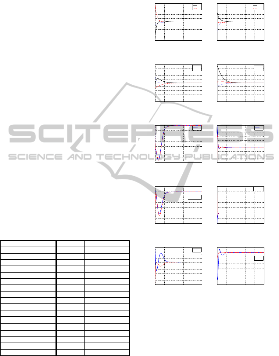
The simulation results for the controller part are
given in figures 4- 7. We see that the inertial positions
and the Euler angles converge in a small neighbor-
hood of zero. Figure 8 shown the control force τ
u
, τ
w
and the control torque τ
r
needed for stabilizing. It is
clear that the total ROV model (14) is locally asymp-
totically stable at the origin using only three control
inputs (15).
Table 1: Rigid Body and Hydrodynamics Parameters.
Parameter Symbol Value
mass m 10.84
moment of inertia I
xx
, I
yy
, I
zz
0.065, 0.216, 0.2
Added mass in surge X
˙u
-1.0810
Added mass in sway Y
˙v
-0.3848
Added mass in heave Z
˙w
-0.3.848
Added inertia in roll K
˙p
0
Added inertia in yaw N
˙r
-0.0075
Added inertia in pitch M
˙q
-0.0075
Surge linear drag d
u
0.9613
sway linear drag d
v
2.4674
heave linear drag d
w
2.4674
yaw linear drag d
r
5.3014× 10
−3
Surge linear drag d
q
5.3014× 10
−3
Added inertia X
˙q
1.0885
Added inertia Y
˙p
0.3848
center of mass G (0,0,-0.16)
center of buoyancy b (0,0,0)
0 1 2 3 4 5
−0.5
−0.4
−0.3
−0.2
−0.1
0
0.1
0.2
0.3
0.4
0.5
error in position [m]
time[sec]
xhat
yhat
zhat
0 1 2 3 4 5
−0.5
−0.4
−0.3
−0.2
−0.1
0
0.1
0.2
0.3
0.4
0.5
error in orientation [deg]
time[sec]
thetahat
psihat
phihat
Figure 2: Errors in position and orientation.
0 1 2 3 4 5
−0.5
−0.4
−0.3
−0.2
−0.1
0
0.1
0.2
0.3
0.4
0.5
error in angular velocity [deg/s]
time[sec]
qhat
rhat
phat
0 1 2 3 4 5
−0.5
−0.4
−0.3
−0.2
−0.1
0
0.1
0.2
0.3
0.4
0.5
error in linear velocity [m/s]
time[sec]
uhat
vhat
what
Figure 3: Errors in linear and angular velocity.
0 10 20 30 40 50
−0.7
−0.6
−0.5
−0.4
−0.3
−0.2
−0.1
0
actual and estimate x[m]
time[sec]
x
xhat
0 10 20 30 40 50
−0.2
−0.15
−0.1
−0.05
0
0.05
0.1
0.15
0.2
0.25
0.3
actual and estimate z[m]
time[sec]
z
zhat
Figure 4: Actual and estimate position.
0 10 20 30 40 50
−0.3
−0.25
−0.2
−0.15
−0.1
−0.05
0
0.05
actual and estimate theta[deg]
time[sec]
erreur theta
thetahat
0 10 20 30 40 50
−0.1
−0.05
0
0.05
0.1
0.15
0.2
0.25
actual and estimate psi[deg]
time[sec]
psi
psihat
Figure 5: Actual and estimate orientation.
0 10 20 30 40 50
−0.3
−0.25
−0.2
−0.15
−0.1
−0.05
0
0.05
0.1
0.15
0.2
actual and estimate u[m/s]
time[sec]
u
uhat
0 10 20 30 40 50
−0.3
−0.25
−0.2
−0.15
−0.1
−0.05
0
0.05
actual and estimate w[m/s]
time[sec]
w
what
Figure 6: Actual and estimate linear velocity.
6 CONCLUSIONS
In this paper, an observer based controller is designed
in order to estimate the state dynamics and to stabilize
the whole closed loop system. The controller observer
is designed based on the Lyapunov technics for non-
linear systems. The particularity of this work is that
the considered system is not in triangular form and its
dynamics are also coupled. The simulation result has
demonstrated the effectiveness of our observer based
Observer-basedcontrollerDesignforRemotelyOperatedVehicleROV
205
0 10 20 30 40 50
−0.1
−0.08
−0.06
−0.04
−0.02
0
0.02
0.04
0.06
0.08
0.1
actual and estimate q[deg/s]
time[sec]
q
qhat
0 10 20 30 40 50
−0.2
−0.15
−0.1
−0.05
0
0.05
0.1
0.15
0.2
actual and estimate r[deg/s]
time[sec]
r
rhat
Figure 7: Actual and estimate angular velocity.
0 10 20 30 40 50
−1.5
−1
−0.5
0
0.5
1
1.5
2
2.5
control [N]
time[sec]
tau1
tau2
tau3
Figure 8: Control surge force, heave force and yaw torque.
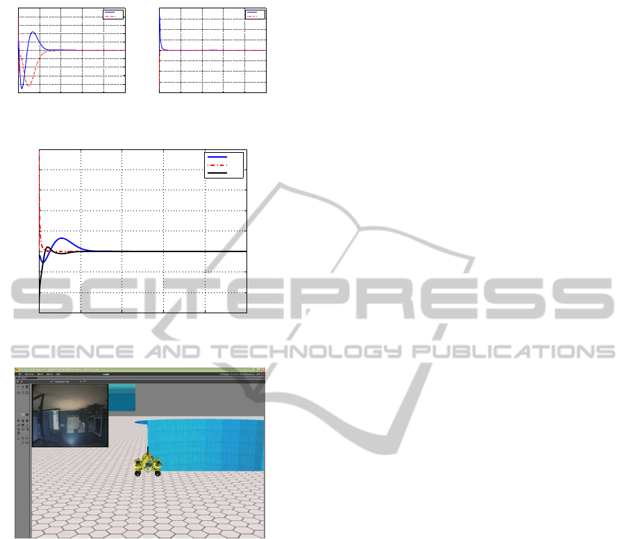
Figure 9: The ROV in virtual subsea.
controller.
In future papers, we will try to test the proposed
work on a simulator while it progresses in a virtual
subsea environment (Fig.9).
ACKNOWLEDGEMENTS
This work is supported by the European Digital Ocean
project under grant FP7 262160.
REFERENCES
Arcak, M. (2002). Observer-based backstepping with weak
nonlinear damping. In American Control Conference,
volume 5, pages 3478–3483.
Berghuis, H. and Nijmeijer, H. (1993). A passivity approach
to controller-observer design for robots. IEEE Trans-
actions on Robotics and Automation, 9:740–754.
Chang, W.-J. and Chen, P.-H. (2013). Stabilization for
truck-trailer mobile robot system via discrete lpv t-s
fuzzy models. In Intelligent Autonomous Systems 12,
volume 193, pages 209–217.
Dounia, S., Mohammed, C., Salim, L., and ThierryMarie,
G. (2012). Robust h
∞
static output feedback stabiliza-
tion of t-s fuzzy systems subject to actuator saturation.
International Journal of Control, Automation and Sys-
tems, 10(3):613–622.
F. Rezazadegan, K. S. and Chatraei, A. (2013). Design of an
adaptive nonlinear controller for an autonomous un-
derwater vehicle. 2:1–8.
Fossen, T. I. (1994). Guidence and Control of Ocean Ve-
hicules. Chichester: Wiley.
Fridman, L., Shtessel, Y., Edwards, C., and Yan, X.-G.
(2008). Higher-order sliding-mode observer for state
estimation and input reconstruction in nonlinear sys-
tems. International Journal of Robust and Nonlinear
Control, 18(4-5).
Gauthier, J.-P., Hammouri, H., and Othman, S. (1992). A
simple observer for nonlinear systems applications to
bioreactors. IEEE Transactions on Automatic Control,
37:875–880.
Gauthier, J. P. and Kupka, I. A. K. (1994). Observability
and observers for nonlinear systems. SIAM J. Control
Optim., 32:975–994.
Kazantzis, N. and Kravaris, C. (1997). Nonlinear observer
design using lyapunov’s auxiliary theorem. In the 36th
IEEE Conference on Decision and Control, volume 5,
pages 4802–4807.
Khadhraoui, A. Beji, L., Otmane, S., and Abichou, A.
(2013). Explicit homogenous time varying stabiliz-
ing control of a submarine rov. In International Con-
ference on Informatics in Control, Automation and
Robotics, (ICINCO 2013), volume 6, pages 26–32.
Khalil, H. K. (2002). Nonlinear Systms. Prentice Hall, third
edition.
Langelaan, J. W. (2006). State Estimation for Autonomous
Flight in Cluttered Environments. phd, Stanford Uni-
versity, Stanford, CA 94305.
Li, J. and Qian, C. (2006). Global finite-time stabilization
by dynamic output feedback for a class of continuous
nonlinear systems. IEEE Transactions on Automatic
Control, 51:879–884.
Li, Y., Xia, X., and Shen, Y. (2011). A high-gain-based
global finite-time nonlinear observer. In 9th IEEE
International Conference on Control and Automation
(ICCA), pages 483–488.
Li, Y., Xia, X., and Shen, Y. (2013). A high-gain-based
global finite-time nonlinear observer. International
Journal of Control, 86:759–767.
Pourgholi, M. and Majd, V. J. (2012). Robust adaptive ob-
server design for lipschitz class of nonlinear systems.
6(3):29 – 33.
Rigatos, G. G. (2012). Nonlinear kalman filters and parti-
cle filters for integrated navigation of unmanned aerial
vehicles. Robot. Auton. Syst., 60:978–995.
ICINCO2014-11thInternationalConferenceonInformaticsinControl,AutomationandRobotics
206

Shen, Y., Huang, Y., and Gu, J. (2011). Global finite-
time observers for lipschitz nonlinear systems. IEEE
Transactions on Automatic Control, 56:418–424.
Takagi, T. and Sugenou, M. (1985). Fuzzy identification of
systems and its applications to modeling and control.
15:116–132.
APPENDIX A
Under the assumption 2.2, the inertia matrix takes the
form (Fossen, 1994)
M =
m
11
0 0 0 m
15
0
0 m
22
0 0 0 0
0 0 m
33
0 0 0
0 0 0 m
44
0 0
m
51
0 0 0 m
55
0
0 0 0 0 0 m
66
where m
11
= m − X
˙u
, m
22
= m −Y
˙v
, m
33
= m − Z
˙w
m
44
= I
x
− K
˙p
m
55
= I
y
− M
˙q
, m
66
= I
z
− N
˙r
m
15
= m
51
= mz
G
− X
˙q
and m
24
= m
42
= −mz
G
−Y
˙p
.
APPENDIX B
These parameters of the linearized system 17 are
given by:
α
1
=
m
55
d
u
m
11
m
55
− m
2
15
α
2
=
m
−15
d
q
m
11
m
55
− m
2
15
α
3
=
m
55
(F
W
− F
B
) − m
15
z
g
F
B
m
11
m
55
− m
2
15
β
1
=
m
11
d
q
m
11
m
55
− m
2
15
β
2
=
m
−15
d
u
m
11
m
55
− m
2
15
β
3
=
m
11
z
g
F
B
− m
15
(F
W
− F
B
)
m
11
m
55
− m
2
15
γ
1
=
Z
w
m
33
, γ
2
=
−(F
W
− F
B
)
m
33
ρ =
d
r
m
66
APPENDIX C
Lemma 6.1. (Young’s inequality) For a, b ≥ 0 and
p, q ≥ 1 such that
1
p
+
1
q
= 1, one has
• ab ≤
a
p
p
+
b
q
q
• If p = q = 2, then, ab ≤
a
2
2ε
+
εb
2
2
, ∀ε > 0
To prove (22) we use Young’s inequality to con-
clude that for any ε
′
i
> 0,
ϖ
1
xu ≤
ϖ
2
1
4ε
′
1
| x |
2
+ε
′
1
| u |
2
ϖ
2
θq ≤
ϖ
2
2
4ε
′
2
| θ |
2
+ε
′
2
| q |
2
ϖ
3
xθ ≤
ϖ
2
3
4ε
′
3
| x |
2
+ε
′
3
| θ |
2
ϖ
4
xq ≤
ϖ
2
4
4ε
′
4
| x |
2
+ε
′
4
| q |
2
ϖ
5
θu ≤
ϖ
2
5
4ε
′
5
| θ |
2
+ε
′
5
| u |
2
ϖ
6
uq ≤
ϖ
2
6
4ε
′
6
| u |
2
+ε
′
6
| q |
2
ϖ
7
zw ≤
ϖ
2
7
4ε
′
7
| z |
2
+ε
′
7
| w |
2
ϖ
8
ψr ≤
ϖ
2
8
4ε
′
8
| ψ |
2
+ε
′
8
| r |
2
(29)
Then, the parameters of the function
˙
V
1
in (22) are
given by:
ε
1
= ε
′
1
+ ε
′
5
+
ϖ
2
6
4ε
′
6
ε
2
=
ϖ
2
1
4ε
′
1
+
ϖ
2
3
4ε
′
3
+
ϖ
2
4
4ε
′
4
ε
3
= ε
′
2
+ ε
′
4
+ ε
′
6
ε
4
= ε
′
3
+
ϖ
2
2
4ε
′
2
+
ϖ
2
5
4ε
′
5
ε
5
= ε
′
5
, ε
6
=
ϖ
2
1
4ε
′
5
ε
7
= ε
′
7
, ε
8
=
ϖ
2
1
4ε
′
7
(30)
Observer-basedcontrollerDesignforRemotelyOperatedVehicleROV
207
