
A Novel Approach to Model Design and Tuning through Automatic
Parameter Screening and Optimization
Theory and Application to a Helicopter Flight Simulator Case-study
Matteo Hessel
1
, Francesco Borgatelli
2
and Fabio Ortalli
2
1
Engineering of Computing Systems, Politecnico di Milano, Piazza Leonardo Da Vinci 32, Milano, Italy
2
TXT Next, TXT e-solutions, Via Frigia 27, Milano, Italy
Keywords: Model Tuning, Screening, Optimization, Machine-Learning, Adaptive Hill-Climbing, Sequential Masking.
Abstract: The aim of this paper is to describe a novel methodology for model-design and tuning in computer
simulations, based on automatic parameter screening and optimization. Simulation requires three steps:
mathematical modelling, numerical solution, and tuning of the model’s parameters. We address Tuning
because, at the state-of-the-art, the development of life-critical simulations requires months to appropriately
tune the model. Our methodology can be split in Screening (identification of the relevant parameters to
simulate a system) and Optimization (search of optimal values for those parameters). All techniques are
fully general, because they leverage ideas from Machine-Learning and Optimization Theory to achieve their
goals without directly analysing the simulator’s mathematical model. Concerning screening, we show how
Machine-Learning algorithms, based on Neural Networks and Logistic Regression, can be used for ranking
the parameters according to their relevance. Concerning optimization, we describe two algorithms: an
adaptive hill-climbing procedure and a novel strategy, specific for model tuning, called sequential masking.
Eventually, we show the performances achieved and the impact on the time and effort required for tuning a
helicopter flight-simulator, proving that the proposed techniques can significantly speed-up the process.
1 INTRODUCTION
Computer simulations have been one of the major
breakthroughs in the 20
st
century technology, with
previously unforeseeable theoretical and practical
implications. Simulations have shown how the
interaction among different entities/components with
non-trivial behaviour can result in an apparently
unpredictable dynamics, opening new perspectives
in the study of complex systems. In countless fields
of Science it is now a standard to resort to
simulations in order to test hypothesis or in order to
get a deeper insight in the dynamics of systems with
sensitive dependency on the initial conditions.
Concerning Engineering, simulations are essential
for both Testing and Training, and increasingly take
the place of traditional experimenting and
prototyping; this has dramatic impact on all
industries where safety and costs are critical factors
(such as the aerospace, bio-medical, pharmaceutical,
and military industries), and makes the development
of highly accurate simulators a life-critical activity.
For a very long time the Modelling and Simulation
techniques were developed independently by
different communities of Civil, Aerospace and Bio-
medical Engineers, and this led to much confusion
and lack of communication, hindering the
development of the sector. Only recently M&S was
recognized as a field on its own, with a well-
established methodology. In order to develop
effective and accurate computer simulations of
complex systems, three main steps are required:
1) Mathematical modelling of the agent(s), of the
environment, of the interactions between agents or
between agent and environment; 2) Numerical
solution of the model’s equations; 3) Tuning of the
model’s parameters. Much work has been done since
the 50s regarding the first steps. Depending on the
kind of simulation, Mathematical Modelling can rely
on principled results from Physics, Operational
Research and Game theory. Concerning the
Numerical solution of the model, beside to domain-
specific approaches (designed for particular
problems in CFD or computational electronics), also
efficient general-purpose techniques are now
24
Hessel M., Borgatelli F. and Ortalli F..
A Novel Approach to Model Design and Tuning through Automatic Parameter Screening and Optimization - Theory and Application to a Helicopter Flight
Simulator Case-study.
DOI: 10.5220/0005022600240035
In Proceedings of the 4th International Conference on Simulation and Modeling Methodologies, Technologies and Applications (SIMULTECH-2014),
pages 24-35
ISBN: 978-989-758-038-3
Copyright
c
2014 SCITEPRESS (Science and Technology Publications, Lda.)

available (e.g. FEM). Thanks to the advances in
these two steps it is therefore possible to model and
solve problems from virtually any application
domain. The third step of M&S, essential whenever
high accuracy is to be achieved, is Tuning; this is the
process of assigning precise values to the free
parameters of the mathematical model behind a
simulation (Even when it is possible to identify the
form of the functional relation among the different
variables of the system, it is seldom possible to set a
priori the exact values of all parameters). Tuning has
not seen in recent years the same development of the
first two steps of M&S, and is often the bottle-neck
of the process of building a simulator. This is the
case, for example, in the flight-simulators industry,
where tight regulatory constraints require a long
Tuning process in order to Certificate a simulator for
pilot Training; however, flight-simulations are not
the only example, and model tuning is even more
crucial in various medical contexts, such as
simulation-driven training (Morgan et al, 2006) and
accurate dose calculation in radiotherapy (which
relies on the ability of precisely modelling the
patient geometry using Computed Tomography
(Lewis et al, 2009)). In all these fields, the complex
tuning job is mostly carried out by hand, using a
trial and error approach in order to modify the huge
number of parameters until the required accuracy is
attained. This approach makes tuning a human-
intensive and time-consuming process (given the
high dimensionality of the solution space and the
complex interactions among parameters) and calls
for the development of automatic tools for model
tuning. In the following sections we begin formally
defining the tuning problem (section 2) and
providing a two-step decomposition of the problem,
heart of the proposed approach (section 3). In
sections 4 and 5 we present automatic techniques for
parameter Screening (i.e. identification of the most
relevant parameters for the effective simulation of a
system) and parameter Optimization (i.e. search of
the optimal values for those parameters); for each
step the state-of-the-art is discussed, highlighting the
major limits of currently used approaches, and
different alternatives are proposed, evaluating pros
and cons of each choice. Finally (section 6) we
validate the proposed techniques against a
Helicopter-simulator case study, comparing the
performances of our two-step approach with manual
tuning (taking TXT e-solutions data as benchmark):
we provide detailed results showing how the
combination of Screening and Optimization can
outperform manual tuning, in terms of speed,
accuracy and capability of dealing with high-
dimensional parameter spaces. It is important to
notice that, although validated against a specific type
of simulation, the proposed methodology is designed
to be as general as possible: our approach leverages
ideas from Machine-Learning and Optimization
Theory in order to achieve its goals treating the
simulator as a black-box, without relying on any
kind of domain knowledge or other a priori
assumptions.
2 THE TUNING PROBLEM
We now give a formal definition of the problem we
are facing, defining the terminology and notations to
be used in the rest of the paper; the elements here
presented can be specialized, depending on the
problem at hand; in section 6 we will see a
specification of all the following for a helicopter
flight simulator (case-study for validation). Let:
- P be a set of n parameters;
- A∈
be a generic assignment of parameters in P;
- Assign to each p
i
∈P a range
,
;
- An assignment A is said consistent if
∈
∀;
- A
0
denotes the initial consistent assignment,
randomly chosen or theoretically derived;
- Let S be a set of domain-specific performance
metrics, measuring different features of the output;
- S(A) represents the values of the performance
metrics computed when the simulation is executed
with the parameters’ assignment A;
- Ref is the set of expected values for the metrics
(ground-truth from observations);
- E(A) is a measure of the global simulation error
(combining errors on the different metrics).
→ The (full) tuning problem is the problem of
finding a consistent assignment A ∈
of all
parameters in P, such that the simulation error E(A)
is minimum.
3 PROPOSED METHODOLOGY
As previously anticipated, the proposed
methodology decomposes the full tuning problem in
two sub-tasks. The two sub-problems can be solved
in sequence, exploiting the results of the first phase
in order to complete more efficiently the second:
→ The screening problem is the problem of ranking
the parameters according to their relevance and
defining a subset SP⊂P of most relevant parameters.
→ The restricted tuning problem requires to find the
ANovelApproachtoModelDesignandTuningthroughAutomaticParameterScreeningandOptimization-Theoryand
ApplicationtoaHelicopterFlightSimulatorCase-study
25

best consistent assignment A|
SP
of parameters in SP,
exploiting the ranking of parameters in SP for
optimization, while assuming fixed the values of all
other parameters (those in P/SP).
If the Screening problem is effectively solved,
the restricted tuning problem should achieve the
same accuracy of the full tuning problem at a lower
cost and introducing less side-effects (issue that will
be explained in more details in section 6, devoted to
experimental results). The techniques for solving the
Screening problem are thus crucial for the entire
proposed approach to tuning.
Figure 1: The flow of the tuning process, highlighting the
available choices for screening and optimization.
4 SCREENING
Screening is a process with a long tradition in classical
statistics, and multiple methods are available to pursue
its goals. Most methods, though, make assumptions on
the distribution of data, require prior knowledge, or
have other disadvantages. One-factor-at-the-time
Designs (Zhang, 2007) require almost no interactions
among factors; Sequential Bifurcation (Bettonvil et al,
1997) requires the sign of the contributes of all factors
to be fixed and known; Pooled ANOVA (Last et al,
2008) requires to know the fraction of relevant factors;
Design Of Experiments (Fisher, 1935) requires to
evaluate an exponential number of configurations,
introducing scalability issues (fractional factorial
designs overcomes this problem through controlled
deterioration of the quality of results; however, the
fraction evaluated must decay with exponential speed
to keep constant the computational resources
required). SB and Pooled Anova assume further a low-
order polynomial relations between input and output
variables, and all previous approaches are usually
based on a two-level scheme (implicitly assuming
linearity - or at least monotonicity - for the functional
form of the output, and making the choice of the 2
levels a sensitive decision). When all assumptions are
satisfied and the required knowledge is available, these
methods can be very effective. However, in our
research, we were looking for a fully general approach
and we considered different Machine Learning
approaches in order to accomplish this goal. Feature
Selection, for example, is the classic area of Machine
Learning dealing with dimensionality reduction and
parameter identification; yet, this is NOT what we are
looking for because F.S. algorithms do not focus on
evaluating the impact of the different parameters on
the simulation’s output, trying just to eliminate
redundancy and relying mostly on learning the
statistical dependencies among factors (which, in our
context, are independent from each other). In order to
exploit Machine Learning for parameter screening we
have followed a completely different track: extracting
a feature ranking from a classifier trained on a
database of previously generated <parameter-set,
simulation error> tuples, and deriving the subset of
relevant parameters from such ranking.
4.1 Database Generation
In order to reduce as much as possible the bias
introduced during this critical phase, the database is
generated randomly using a normal distribution
centred in A
0
. The standard deviation depends on the
range R
i
of each parameter: it is a trade-off between
the necessity of exploration as much as possible of the
solution space and the need of remaining within the
ranges:
,∀1
|
|
(1)
~
0,
,
(2)
|
|
(3)
Assuming the range symmetric with respect to the
initial assignment, with this policy about 1 out of 10
parameters will be sampled outside the range of
SIMULTECH2014-4thInternationalConferenceonSimulationandModelingMethodologies,Technologiesand
Applications
26

feasible values: outlier must be set on the boundary in
order to make all assignments consistent. After the
database set up, a simulation is executed for each
assignment A, and the error E(A) is stored as “class”
variable. The class variable is then discretized
(although this is compulsory only if Logistic
Regression is used in the proceedings). Discretization
can be done through a binomial partition (acceptable-
error, unacceptable-error), or a N bin partition with
equal frequency. Finally, how large must the whole
database be depends on which of the proposed ranking
algorithms is chosen in the following steps and on the
number of parameters (section 6).
4.2 Ranking: Logistic Regression
Logistic Regression (LR) is a classical classification
algorithm, very popular when dealing with discrete
class variables. We now give a brief presentation on
how to apply Logistic Regression and interpret the
results, discussing pros and cons of this choice in the
context of computer simulations. Implementations of
these ideas are available in most data analysis
packages (such as the Matlab Statistical Toolbox, or
its open source alternatives Weka and R). More
detailed information can be found in literature in
(Harrel, 2001) or in (Bishop, 2006).
4.2.1 The LR Model
Logistic Regression is the most famous and widely
used generalized linear model (Nelder et al, 1972)
with link-function given by the famous logit
function:
ln
1
(4)
Given a binomial class variable (Low_Error
High_Error) the LR model is described by the
following equations, where the coefficients grouped
in the vector β
are computed through either
maximum likelihood or maximum a posteriori
estimation:
_
∑
∗
(5)
(6)
_
(7)
The extension to a multinomial model is quite
straightforward; supposing K possible outcomes and
assuming the independence of irrelevant alternatives
a simple way to build the multinomial logit model is
to run independently K-1 binomial logistic
regressions, leaving out just the last outcome Y
K
:
ln
(8)
Then, by exponentiation of both terms, isolating the
different probabilities, and exploiting the fact that
probabilities of all outcomes must sum up to one:
∗
(9)
1
1
∑
(10)
There are many extensions to this model, among
these we point out (Cessie et al, 1992) which uses
ridge estimators to improve accuracy high
dimensional parameter spaces. This slightly
modified Logistic Regression algorithm is the one
implemented in Weka, and the one used in our case-
study (section 6).
4.2.2 Parameter Ranking
If the LR approach is chosen it is easy to extract
measures of relevance for the parameters of the
model: the coefficients of the parameters already
provide such ranking. In general, this is not a
reliable measure if the different factors are highly
correlated, because multi-collinearity makes
computing the relevance of the single covariates
much more complex; therefore more sophisticated
metrics have been developed, which are capable of
producing valid results in such situations (among
these Dominance analysis, Likelihood ratio and
Wald statistics). However, multi-collinearity is not
an issue for us, because in computer simulations the
different parameters are independent and our
database is appropriately built in such manner; thus,
the ranking provided by the coefficients β
i
is
perfectly valid and there is no need to resort to more
complex procedures in order to obtain meaningful
results.
4.2.3 Pros and Cons of LR
The Logistic Regression model can achieve good
classification performance with a relatively low
amount of training data; most potential shortcomings
of this approach, such as the unreliability of the
coefficients as measure of relevance of the single
variables, are due to multi-collinearity, issue that, as
we have seen, is not present in our peculiar context.
The main problem with the use of Logistic
Regression for parameter ranking is that the
functional landscape that can be learned is limited;
therefore, very complex objective functions might
ANovelApproachtoModelDesignandTuningthroughAutomaticParameterScreeningandOptimization-Theoryand
ApplicationtoaHelicopterFlightSimulatorCase-study
27

require more powerful classifiers in order to be
properly modelled and offer a valuable insight on
the relevance of the different parameters. This is the
reason for introducing an alternative approach,
4.3 Ranking: Multilayer Perceptron
The Multilayer Perceptron (MP) is a feedforward
artificial neural network model, widely used in
classification problems, both for discrete and
continuous class variables. Therefore, we can train
the Multilayer Perceptron either on the original
database of simulations or on the version with
discrete class variable used for LR. Detailed
information on this topic can be found in (Haykin,
1998), and implementations of the ideas presented in
sections from 4.3.1 to 4.3.4 can be found in Weka
(Hall et al, 2009), in the RSNNS (Bergmeir, 2012),
and in the Matlab Neural Networks Toolbox. As
done for Logistic Regression, we now briefly
describe the model, discuss pros and cons of its
application to computer simulations, and finally
define the strategy that shall be used for parameter
ranking.
4.3.1 The MP Model
The perceptron was first proposed in (Rosenblatt,
1958) as the simplest model of the behaviour of
biological neurons. The perceptron maps N inputs
into a single binary or real-valued output variable y,
computed applying an activation function f to a
linear combination of the inputs and of a threshold
b, weighted by coefficients w
i
. Common activation
functions are the step function, the sigmoid functions
(such as the logit or the hyperbolic tangent), and the
rectifier/softplus functions.
Figure 2: this figure presents the pipelined structure of a
single perceptron, highlighting its main features.
A perceptron alone is quite limited and cannot be
used for non-linearly separable classification
problems. The combination of many perceptron in
an Artificial Neural Network, is instead extremely
powerful. The Multilayer Perceptron is an acyclic
layered directed graph of perceptrons with non-
linear activation function; the first layer (the input
layer) has |P| nodes, and the last layer (the output
layer) has as many nodes as the number of outcome
variables (for numeric classes) or as the number of
possible values of the outcome variable (for discrete
classes); other layers (called hidden layers) can have
any number of nodes.
Figure 3: the very common three layered MLP
4.3.2 Computation
Given L+1 node-layers (counting input, output and
hidden layers) and L edge-layers (the connection
layers between the node layers), the computation of
a multilayer perceptron can be described as a
sequence of non-linear transformations from x
0
to x
L
:
x
0
,
,
x
1
,
,
…
,
,
x
L
If N
j
is the number of nodes at layer j, x
j
∈
for
all j=0,…,L represents the input of layer j, and W
j
is
an N
j
×N
j-1
matrix for all j=1,…,L whose elements
W
j
h,k
represent the weight of the edge connecting
node h of layer j with node k of the previous layer j-
1. The output value is computed applying in order,
for all edge-layers for j=1 to j=L, the following
expression:
∑
(11)
This paradigm of computation is the reference that
must be kept in mind in order to understand how the
network is trained to learn the weights that best
approximate a target function.
SIMULTECH2014-4thInternationalConferenceonSimulationandModelingMethodologies,Technologiesand
Applications
28

4.3.3 Topology
If a MP model is to be trained on our database, first
the structure of the network must be chosen; the
number of inputs and outputs is fixed thus the main
design choices are the number of hidden layers and
the number of nodes within those layers. The most
widely used network topology has just one hidden
layer. The reason is that convergence is usually
faster for shallow architectures and it has been
proved that the MP with a single hidden layer is a
universal approximator (Cybenko, 1989), thus any
function can be approximated with arbitrary
precision if the weights of edges are properly
chosen. In recent years, though, improvements in the
training of deep networks (Hinton et al, 2006) have
made other choices feasible, and some theoretical
results imply that the universal approximation
property of the three layered MP is achieved at the
cost of an exponential number of nodes with respect
to networks with more hidden layers. Therefore, our
approach to parameter ranking through the analysis
of a trained MP applies to networks with any
number of layers.
4.3.4 Training
Once the network’s topology has been devised, the
best values for the network’s weights must be found,
this is done with the iterative back-propagation
algorithm (Rumelhart, 1986) using the database of
pre-classified simulations. Let t be the iteration (also
called epoch) and η a parameter called learning rate;
if the database with continuous class variable is
used, training proceeds according to the following
rules, applied each iteration to all instances in the
dataset (discrete classes are dealt with likewise): 1)
compute the difference between the expected output
‘ex’ and the actual output ‘x
L
’; 2) propagate the error
across the network from output to input layer; 3)
update the weights and the thresholds values:
′
(12)
∑
1 (13)
∆
,1 (14)
∆
,1 (15)
This algorithm is the most widely used, although
convergence is quite slow it can be made more
efficient resorting to batching and multithreading.
It is proved equivalent to gradient descent applied to
an appropriate cost function and shares therefore the
known limits of such approach: convergence not
guaranteed and result possibly a local optimum.
4.3.5 Parameter Ranking
Extracting measures of relevance from a trained
Multilayer perceptron is a complex task and there is
no single way for doing so. Various approaches have
been proposed in the past, all with their specific pros
and cons; we present an alternative heuristic
approach that is easily applicable to MPs with any
number of hidden layers. Consider a network with
L+1 node-layers and L edge-layers, with a single
continuous outcome variable; given the previously
defined notations, and denoted as R the array of
length || containing the parameters’ ranks:
∶
(16)
…
∏
(17)
If the network was made of linear perceptrons
(having the identity function as activation function),
each element of R would represent exactly the
contribution to the outcome variable of the
associated parameter when it takes unitary value.
When applied to networks of non-linear perceptrons
the metric has just a heuristic value, yet it has
proved itself very effective in our experiments on
flight simulations, yielding to even better results
than LR (see section 6 for more details). The
extension of the method to N outcome variables or
to a discrete outcome having N possible values is
trivial (R is a matrix with obvious meaning).
4.3.6 Pros and Cons of MP
The multilayer perceptron’s main strength is its
representation power, due to its being a universal
function approximator. Furthermore, the MP can be
trained on the original simulation error values, and
does not require discretization as LR, although it is
still possible to train the network on the discretized
dataset. However this approach has one big
disadvantage when applied to our computer
simulated environment: it usually requires a larger
amount of data if compared to Logistic Regression.
This can be a problem because we are responsible of
generating all data to be analysed: computer
simulations can be computationally expensive and it
is not always possible to speed up computation just
adding resources. Indeed, this was the case in our
case-study for validation: being a training flight
simulator, was designed in such a way that
simulations could only be executed in real-time). If a
ANovelApproachtoModelDesignandTuningthroughAutomaticParameterScreeningandOptimization-Theoryand
ApplicationtoaHelicopterFlightSimulatorCase-study
29

single function evaluation (i.e. a single computation
of the simulation error for a given set of parameters)
takes very long we therefore advise to try Logistic
Regression first, and resort to the Multilayer
Perceptron if needed.
4.4 Computing SP
We use feature ranking algorithms to evaluate all
parameters of the model, assigning to each
parameter a weight, measuring its importance.
However in the subsequent phase we do not only
exploit the ranking among different parameters, but
execute the various optimization procedures
allowing them to modify only a subset SP of the
model’s parameters (restricted tuning problem).
Defining which parameters are the “most” relevant
and must be considered for tuning process is
somehow arbitrary, and requires to find a trade-off.
Considering for automatic tuning a high number of
parameter implies the exploration a large solution-
space and might introduce despicable side-effects
(which do not directly influence the performance
metrics but make the simulation less “natural” to a
human eye); Instead, considering a too small set of
parameters might make optimization impossible if
the optimum falls in the portion of spaces that
becomes unreachable once fixed the values of
parameters in P/SP. In order to use the ranks/weights
of parameters to take a good decision, we suggest to
sort the parameters according to their weights and
then draw the cumulative function: the parameter set
can be cut where the slope of the function slows
down and at least a given percentage of the total
weight is reached (e.g. at least 90-95%). An example
of this procedure is shown in section 6 both for the
Logistic Regression and for the Multilayer
Perceptron rankings (figures 5 and 6).
5 OPTIMIZATION
We have now reached the final step: the solution of
the (restricted) tuning problem through automatic
optimization procedures managing only the
parameters in the previously defined subset SP. We
present first a basic stochastic Hill Climbing
procedure (searching for optimal values of all
parameters in SP), then we describe two successive
refinements of the algorithm which have proved
themselves effective in a real tuning case-study. The
first refinement introduces adaptive variance, and
corresponds to a 1+1 evolutionary strategy. The
third algorithms, which is by large the most
efficient, is also capable of exploiting the ranking of
parameters in SP in order to tune an increasing
number of parameters at each iteration.
5.1 Local Optimization, Why?
All proposed approaches are local (and stochastic)
optimization strategies; this is no accident, and it is
appropriate for the following reasons:
1) Do we have any choice? Often we do not; global
optimization is more computationally demanding,
therefore, in M&S, it might simply be impossible.
The time for each function evaluation can be very
long; executing different simulations in parallel can
be unfeasible if all computational power available is
required for executing a single computer simulation;
finally, sometimes, e.g. in real-time simulations, no
speed-up of the single simulation is possible even if
more computational power is available.
2) If modeling is carried out in a sensible way, the
initial assignment A
0
is not a completely random
guess but a reasonable solution derived by physical
considerations, and is thus (hopefully) near to the
true optimal solution making local optimization less
at risk of remaining stuck in non-global optima.
3) When you recreate in a simulator some known
observed reality (which is typical of flight or other
life-critical simulations) you can recognize if you are
stuck in a local optima because you know which the
optimal value is (although you do not know where it
is located within the very large solution-space).
4) Concerning the choice of stochastic optimization
instead of deterministic procedures, there are two
elements to be considered: first, stochastic
procedures are less prone to getting stuck in local
optima, second, most stochastic algorithms needs to
know very little about the function (no need to
compute derivatives or similar). Having devoted so
much time to develop screening techniques capable
of treating the model just as a black box, we do not
want to start analyzing the equations now that
efficient black-box optimization techniques are
readily available.
5.2 Basic Stochastic Hill Climbing
The basic Hill climbing procedure we now present
in pseudo-code shall be thought of as a template to
be refined in the following. Therefore, it’s quite
impressing that, as we will see, even in this basic
form the procedure accomplishes a reasonably low
error, showing the power of Screening in making
tuning possible. The algorithms works exploring the
neighbourhood of the best solution up to a given
SIMULTECH2014-4thInternationalConferenceonSimulationandModelingMethodologies,Technologiesand
Applications
30

moment until a better one is found, then it moves to
the new location and continues:
01 best = A
0
02 A = A
0
03 min-err = execute(A
0
)
04 R = loadRange()
05 σ = computeStdDev(R)
06
07 while (error>threshold)
08
09 for (j=1 to |P|)
10 if(p
J
in SP)
11 A
J
= best
J
,+ σ
J
× N(0,1)
12 A
J
= setWithinRange(A
J
,R
J
)
13 end-if
14 end-for
15
16 if(execute(A) < min-err)
17 min-err = execute(A)
18 best = A
19 end-if
20
21 end-while
best contains the best assignment found up to the
current iteration, min-err storing the corresponding
error. Exploration of the neighbourhood of best is
random: new assignments of each parameter
in
SP are generated each iteration sampling from a
normal distribution centred in
. The function
computeStdDev(R) defines once for all the
value of the standard deviation used for each
parameter
, which is proportional to the range
;
the same precautions seen for the database
generation, to guarantee the consistency of all
assignments, are taken into account also in this
circumstance when defining the relation between
range and standard deviation (section 4.1). Function
execute(A) runs the simulation with
parameters’ values specified by A and computes the
simulation error E(A). Note that, as required, all
parameters in P/SP maintain their initial default, and
that as the number of iterations grows to infinity the
best parameter assignment eventually converges to
the global optimum with probability 1.
5.3 Adaptive Variance
In the hill climbing procedure of the previous
section, random mutations occur every iteration in
order to explore the neighborhood of the best
solution found; the parameter controlling such
mutations is the standard deviation of the normal
distribution used for sampling. As it is, this standard
deviation could be computed statically, depending
only on the range of the different parameters
considered; however, the optimal value of σ is not
the same throughout the execution of the
optimization procedure: indeed, it is intuitively clear
that the best value for σ should be greater when the
error is high and we are exploring the solution space
with a high success rate, while it should become
increasingly smaller when we are very near to the
optimum and very small corrections are needed in
order to improve our solution. This calls for a crucial
important modification of the procedure of section
5.1, allowing σ to adapt on-line during optimization.
There are two main approaches to achieve the
required capability: make the standard deviation
decrease along with the simulation error, or make it
increase or decrease dynamically depending on the
success rate (the fraction of mutations that are
successful, i.e. that improve the best solution). The
former approach still requires to define at design-
time the exact relation between error and standard
deviation, instead the latter is usually more powerful
because provides greater flexibility. A common
policy when the second approach is chosen is to
decrease σ when the success rate is below 0.2 and
increase it otherwise (this strategy is known as the
1/5 success rule; it can be proved optimal for several
functional landscapes and it is widely recognized to
give good results in practice in a wide range of
circumstances). Among the many implementations
of such rule, the simplest one (Kern et al, 2004)
accumulates the knowledge about success and
failure directly in the value of σ, substituting the if-
else clause of lines 16-19 with the following code:
18 if(execute(A) < min-err)
19 min-err = execute(A)
20 best = A
21 σ
J
= σ
J
α
22 else
23 σ
J
= σ
J
/
24 end-if
Reasonable values of parameter α are between
2
/
and 2. This implementation requires to set only
1 parameter instead of the 3 (change rate, averaging
time to measure success rate, update frequency)
needed with classical implementations following
more narrowly the previous definition.
5.4 Sequential Masking
Although the hill climbing procedure, modified in
order to adapt online the parameter controlling the
entity of mutations, can already be used in practice
to solve the restricted tuning problem, performance
ANovelApproachtoModelDesignandTuningthroughAutomaticParameterScreeningandOptimization-Theoryand
ApplicationtoaHelicopterFlightSimulatorCase-study
31

can be further improved by the third algorithm,
Sequential masking, exploiting the ranking of
parameters in SP. This third approach to automatic
tuning works as follows:
1) A sequence of subsets, and thus of restricted
tuning problems, SP
1
SP
2
… SP is generated
incrementally from the ranking of parameters in SP.
2) the hill climbing procedure with adaptive variance
is executed for a fixed number of iterations for each
sub-problem, starting from the smallest (simplest)
problem and using the result of each problem as
initial guess of the subsequent problem.
Figure 4: Sequential masking with four sub-problems.
The idea is that challenges of increasing complexity
are faced starting from increasingly good initial
assignments. The increasing complexity is due to the
fact that an increasing portion of the solution space
is reachable. In conclusion, as shown in figure 4,
starting from assignment A
0,
we compute a sequence
of solutions converging to the final solution
of
the restricted tuning problem with parameters SP.
→
→
…
→
→
...
→→
The execution of the algorithm is controlled by two
user defined parameters: the number of restricted
tuning problems, which we can call the granularity
of the algorithm, and the maximum number of
iterations for each phase of the procedure. The max
number of iteration can be different for each of the
problems (higher for those considering more
parameters).
6 CASE-STUDY
Our case-study for validation is the tuning of an
industrial level flight-simulator of our_company in
order to accurately simulate the take-off of a
helicopter with one engine inoperative (breaking
down during the execution of the procedure). This
case-study is a classic example of simulator with
severe accuracy requirements, as flight simulators
must be certificated by flight authorities of different
countries, verifying that the execution of a certain
set of flight procedures is adherent to the observed
behavior of the aircraft. There are 2 main procedures
for take-off: Clear area TO and Vertical TO. We
here analyse only the clear area procedure, showing
the results of the screening and optimization
algorithms (however the techniques have been
applied to both). In the following P is a set of 47
parameters, each associated to a range symmetric
with respect to the initial assignment A
0
. The
relevant performance metrics in S are three: CTO
distance (distance from starting point to take-off-
decision-point), GP1 (average climb in 100 feet of
horizontal motion during the 1
st
phase), and GP2
(average climb in 100 feet of horizontal motion
during the 2
nd
phase). Expected values Ref of such
metrics are specified on the helicopter’s official
manual. The global error E(A) is the sum of the
squared relative errors with respect to the three
performance metrics.
6.1 Screening
A database of 1200 simulations has been generated
with the rules established in section 4.1,
appropriately discretizing the values of the global
simulation error. Then both the logistic regression
and the neural network based approach to parameter
ranking are applied, using the implementations
available in the open source machine-learning
package Weka (And choosing the classic three
layered topology for the MP). Results were largely
consistent: if the set of 10-20 most relevant
parameters for LR is compared to the corresponding
set within the MP ranking, about, about 85% of the
parameters figure in both sets. The main difference
is a single small group of parameters, having similar
physical meaning, in which all parameters are
ranked very low by LR while MP seems to be able
to discriminate more effectively between relevant
and not relevant parameters. If the cumulative
functions of the two approaches are compared
(Figure 7 and 8), this difference among the results is
reflected in a steeper curve for the LR-based
ranking, which concentrates most of the weight on
fewer parameters (trend confirmed by other flight
procedures). The resulting set SP of the most
relevant parameters is thus smaller for LR than it is
for MP.
SIMULTECH2014-4thInternationalConferenceonSimulationandModelingMethodologies,Technologiesand
Applications
32

Figure 5: Cumulative weight-function, LR ranking.
Figure 6: Cumulative weight-function, MP ranking.
6.2 Evaluating Screening
In the next section we will go into details in the
comparison of the performances of adaptive hill
climbing and sequential masking, but, before, we use
the basic optimization procedure in order to provide
the reader with an intuitive proof of the impact of
the previous screening techniques; In figure 7 four
executions of the basic HC procedure are compared;
the horizontal axis identifies the number of
simulations executed, while the vertical axis
measures the minimum error up to the given
iteration. In all four cases the algorithm has gone
through 100 iteration: the solid lines represent the
execution of the algorithm considering the results of
screening (through LR and MP respectively); the
dotted line, that converges to a relatively high
simulation error and then stops improving, represent
the execution of the procedure with SP=P (i.e. the
procedure if applied directly to the full tuning
problem with no screening); the dashed line, that
shows no improvements at all, represent the
execution using only parameters in P/SP
Figure 7: Execution of the basic hill climbing optimization
with different screening policies.
In conclusion, figure 7 shows that LR and MP based
rankings truly identify the relevant parameters: if
optimization is allowed to modify only low-ranked
parameters no improvement is achieved; if instead
only high-ranked parameters can be modified, the
restricted tuning problem is solved faster than the
full problem and a lower error is reached: the
algorithm with P=SP keeps an acceptable rate only
for the first 10 iterations, then it almost stops and
maintains a constant almost imperceptible
improvement rate.
6.3 Optimization
We now show the results of applying the two
proposed optimization algorithms to our case-study.
Both converge to an error many orders of magnitude
lower than the one achieved by the basic hill
climbing procedure, and they also do so significantly
faster. In order to make the results understandable
the vertical axis is now the (base 10) logarithm of
the error.
The comparison of the two algorithms in figure 8
shows that they both are able to keep the error
decreasing at a good, almost constant, average rate.
Sequential masking achieves particularly impressive
performances, however both algorithms proved
themselves effective, significantly improving the
basic Hill climbing procedure, in figure 7, which
instead, whether screening is used or not, hits sooner
or later a wall, becoming unable of further
improvements, or capable of doing so only at an
unacceptable slow rate.
ANovelApproachtoModelDesignandTuningthroughAutomaticParameterScreeningandOptimization-Theoryand
ApplicationtoaHelicopterFlightSimulatorCase-study
33
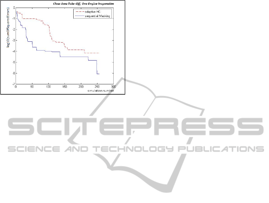
Figure 8: Comparison of sequential masking and adaptive
hill climbing optimization procedures.
6.4 Benchmarks and Conclusions
In conclusion our approach has been proved
effective in tuning a complex flight simulation
model finding the optimal values of 50 parameters
of the model. The entire process requires less than 2
days of machine-time on a single desktop computer
(with just a few hours actually dedicated to finding
those values, and most of the time devoted to
generating the database for parameter ranking). The
main benchmark against which this result must be
compared is manual tuning, which is still the state-
of-the-art in industrial applications. Our_company’s
experienced engineers would require from 10 to 20
days to accomplish the same result. Concerning
previous attempts to automatic tuning, there is little
work done for the tuning of industrial level
computer simulators, and to the best of our
knowledge, none in the area of flight simulations.
The best related work is in medical context (Vidal et
al, 2013): this paper presents an evolutionary
strategy for tuning, but the approach is used only for
lower dimensional problem with just 15 parameters.
Thanks to an integrated approach combining
screening and optimization (tightly coupled
especially in the sequential masking algorithm), our
methodology allows to significantly expand the
range of application of automatic techniques for
parameter tuning. When comparing to other attempt
of automatic tuning it is important to notice that
combining screening and optimization is not only
crucial in order to achieve fast convergence to a
really low simulation error, but it is also crucial in
order to avoid an issue we have anticipated in
previous sections of the paper: the introduction of
peculiar side effects that can make simulations
unrealistic to a human eye (such as odd small
oscillations and vibrations difficult to control). The
reason for such side-effects is that parameters that
have a low impact on the performance metrics and
thus on the global simulation error are free to deviate
randomly from their default values, because there is
no selective pressure capable of limiting their erratic
wandering. Our methodology solves the issue by
restricting tuning to the set of parameters with direct
impact on the performance metrics, so, during
optimization, all non-fixed parameters are directed
towards their optimal values instead of being free to
roam around. The proposed methodology is
therefore the first real alternative to manual tuning,
allowing an impressive speed up of the tuning
process while preserving high quality results.
Having applied the machine learning algorithms
without exploiting any prior domain knowledge we
also believe that is fully general, as future research it
would be therefore interesting to apply the proposed
technique to other application domains.
REFERENCES
Fisher, R.A., 1935, The design of experiments. Oxford,
England: Oliver & Boyd. xi 251 pp.
Rosenblatt F., 1958, The perceptron: a probabilistic model
for information storage and organization in the brain.
Psychological Review 65: 386—408.
Nelder J., Wedderburn R., 1972 Generalized Linear
Models, Journal of the Royal Statistical Society. Series
A (General) 135 (3): 370-384.
Rumelhart D.E., Hinton G.E., Williams R.J., 1986,
Learning representations by back-propagating errors.
Nature 323 (6088): 533–536. doi:10.1038/323533a0.
Cybenko G., 1989 Approximations by superpositions of
sigmoidal functions, Mathematics of Control, Signals,
and Systems, 2 (4), 303-314.
Le Cessie S., Van Houwelingen J.C., 1992, Ridge
estimators in Logistic Regression. Applied Statistics.
Bettonvil B., Kleijnen J.P.C., 1997, Searching for
important factors in simulation models with many
factors: Sequential bifurcation, European Journal of
Operational Research, Volume 96, Issue 1, Pages 180–
194.
Haykin S., 1998, Neural Networks: A Comprehensive
Foundation (2 ed.). Prentice Hall. ISBN 0-13-273350-
1.
Harrel F., 2001 Regression Modeling Strategies, Springer-
Ve rl ag .
Kern S., Muller S.D., Hansen N., Büche D., Ocenasek J.,
Koumoutsakos P., 2004, learning probability
distributions in continuous evolutionary strategies – a
comparative review, Journal of Natural Computing
Volume 3 Issue 1, Pages 77 - 112.
Bishop C., 2006 Pattern Recognition and Machine
Learning, Springer Science+Business Media, LLC, pp
SIMULTECH2014-4thInternationalConferenceonSimulationandModelingMethodologies,Technologiesand
Applications
34

217-218.
Hinton G.E., Osindero S., Yee-Whye The, 2006, A fast
learning algorithm for deep belief nets, Neural
Computation, 18(7):1527–1554.
Morgan P.J., Cleave-Hogg D, Desousa S., Lam-
McCulloch J., 2006, Applying theory to practice in
undergraduate education using high fidelity
simulation, Med Teach, vol. 28, no. 1, pp. e10–e15.
Zhang A., 2007 One-factor-at-a-time Screening Designs
for Computer Experiments, SAE Technical Paper
2007-01-1660, doi:10.4271/2007-01-1660.
Last M., Luta G., Orso A., Porter A., Young S., 2008,
Pooled ANOVA, Computational Statistics & Data
Analysis, Volume 52, Issue 12, Pages 5215-5228.
Hall M., Eibe F., Holmes G., Pfahringer B., Reutemann P.,
Witten I., 2009 The WEKA Data Mining Software: An
Update; SIGKDDExplorations, Volume11, Issue1.
Lewis J. H., and Jiang S. B., 2009, A theoretical model for
respiratory motion artifacts in free-breathing CT
scans, Phys Med Biol, vol. 54, no. 3, pp. 745–755.
Bergmeir C., Benìtez J.M., 2012, Neural Networks in R
Using the Stuttgart Neural Network Simulator:
RSNNS, Journal of Statistical Software, Volume 46,
Issue 7.
Vidal F.P., Villard P., Lutton E., 2013, Automatic tuning of
respiratory model for patient-based simulation,
MIBISOC’13 - International Conference on Medical
Imaging using Bio-inspired and Soft Computing.
ANovelApproachtoModelDesignandTuningthroughAutomaticParameterScreeningandOptimization-Theoryand
ApplicationtoaHelicopterFlightSimulatorCase-study
35
