
A Navigational Framework Combining Visual Servoing and Spiral
Obstacle Avoidance Techniques
Marcus Futterlieb
1,2
, Viviane Cadenat
1,2
and Thierry Sentenac
1
1
CNRS, LAAS, 7 avenue du Colonel Roche, F-31400 Toulouse, France
2
Univ de Toulouse, UPS, LAAS, F-31400 Toulouse, France
Keywords:
Navigation, Control, Mobile Robotics, Visual Servoing, Navigational Framework, Obstacle Avoidance.
Abstract:
This paper presents a navigational framework which enables a robot to perform Long Range Navigation in the
context of the Air-Cobot-Project in which a robot is used to execute an autonomous pre-flight inspection on
an aircraft. The robot is equipped with Laser range finders and a mobile stereo camera system. The idea is to
guide the robot to the pre-defined checkpoints using a Visual Servoing controller based on video data, while
avoiding static and moving obstacles. The contribution of the paper is an avoidance technique derived from
the spiral flight path of insects applied to the Laser range data. Simulation results validate the whole approach.
1 INTRODUCTION
In mobile robotics, especially for industrial robots, it
is very important to have a robust and reliable naviga-
tion strategy to guide the robot through its workplace.
With human workforce in its vicinity it is necessary to
keep the robot in a caged environment or alternatively
equip it with some sort of obstacle avoidance (OA).
The objective of Air-Cobot-Project is to design, de-
velop and evaluate a robot able to assist or solely in-
spect an aircraft before takeoff and provide diagnosis.
Therefore, the robot has to move autonomously be-
tween different checkpoints while taking into account
the presence of both men and vehicles in its vicinity.
It also must be collaborative with the airport informa-
tion systems.
Thus, the robot has to perform a long range nav-
igation assignment which involves several tasks re-
spectively related to perception, environment model-
ing, localization, path planning and supervision which
will be coupled within a navigational framework. In
the project, the perception task is based on both cam-
eras and laser sensors. A modeling task provides
the metric and the topologic maps describing the air-
port environment with the different checkpoints to be
reached successively. Path planning has to compute
a path allowing the robot to reach the aircraft inspec-
tion site starting from its initial position. Furthermore,
the localization method has to provide the pose of the
robot relatively to the aircraft and to a global fixed
frame. The robot’s motion will be determined by a
supervisor, a high level controller, which will choose
the most appropriate controller depending on the con-
text. In our case, several controllers will be available:
a trajectory following controller allowing to reach the
inspection site; a Visual Servoing (VS) controller al-
lowing to reach each checkpoint thanks from visual
data of the aircraft taken by the embedded cameras;
an OA controller ensuring collision free execution of
the task.
Our contribution is related to visual navigation in
possibly cluttered environment, meaning that a cam-
era is used as the main sensor to move the robot to-
wards the goal. To do so we can use either global or
local approaches. Generally speaking, global meth-
ods assume that the robot is provided a map prior to
the navigation. With the help of this map long range
displacements are conceivable. However, as this map
can only take into account obstacles which are known
a priori it must be updated whenever new objects
arise. These techniques appear to introduce some
rigidity in the navigation system even if improve-
ments have been made by developing methods al-
lowing to re-plan a new path (Koenig and Likhachev,
2005) (Lamiraux et al., 2004) or to locally modify the
robot’s trajectory (Owen and Montano, 2005) (Damas
and Santos-Victor, 2009).
On the contrary, local methods do not require a
map, meaning that obstacles do not need to be known
a priori but can be detected during the mission. Fur-
thermore, the robot will move through the scene de-
pending on the goal to be reached and on the sen-
57
Futterlieb M., Cadenat V. and Sentenac T..
A Navigational Framework Combining Visual Servoing and Spiral Obstacle Avoidance Techniques.
DOI: 10.5220/0005027800570064
In Proceedings of the 11th International Conference on Informatics in Control, Automation and Robotics (ICINCO-2014), pages 57-64
ISBN: 978-989-758-040-6
Copyright
c
2014 SCITEPRESS (Science and Technology Publications, Lda.)
sory data perceived during the navigation. Some well
known techniques such as potential field (Khatib and
Chatila, 1995) or the VFH* (Ulrich and Borenstein,
2000) technique belong to this category. More recent
works have proposed to couple two controllers allow-
ing to reach the goal and to guarantee non-collision
(Folio and Cadenat, 2005) (Vilca et al., 2013). These
methods tend to be more reactive, but they can suf-
fer from local minima and only allow for short range
displacements.
Therefore, it seems interesting to couple a global
with a local approach to take advantage of both meth-
ods. This is a concept presented in (Matsumoto et al.,
1996) and which has been re-used in (Cherubini et al.,
2013), (Cherubini et al., 2012) and (Adrien D. Pe-
titeville and Cadenat, 2012). To summarize, the ap-
proach consists in defining the path to be followed in
a sequence of images known as visual road. Making
the robot follow this path is achieved with the help of
a VS controller. OA can be performed by coupling a
proper controller to the VS.
In this article we will focus on the design of a new
OA controller in the background of (Adrien D. Pe-
titeville and Cadenat, 2012). For the context of our
project, the robot has to mainly avoid unexpected
static and moving obstacles. It is inspired by an arti-
cle showing that insects perform a spiral path around a
light source (Boyadzhiev, 1999). Following a reason-
ing similar to the one developed in (Mcfadyen et al.,
2012b),(Mcfadyen et al., 2012a) our idea is to adapt
this method to make a robot avoid the obstacle by per-
forming a spiral around a specific point to be defined.
We will provide some guidelines about the choice of
this point and the avoidance control law.
The structure of this article will be the following:
In the next section, we will introduce the necessary
conceptual basics of our work. After that we present
our first theoretical and simulation results about the
obstacle avoidance method and give some results we
have achieved through simulation with the Robot Op-
erating System and Gazebo. Finally we provide a
conclusion.
2 BACKGROUND ON VISUAL
SERVOING AND ROBOT
MODELING
2.1 Description of the Sensors and
Robot
The robot we consider in this project is outfitted with
numerous sensors dedicated to both, Non-destructive
Testing and navigation. In this article we will fo-
cus on the latter one. For navigational purposes, our
robot is equipped with an IMU, a stereo camera sys-
tem mounted on a pan tilt unit (PTU) and a laser range
finder (LRF).
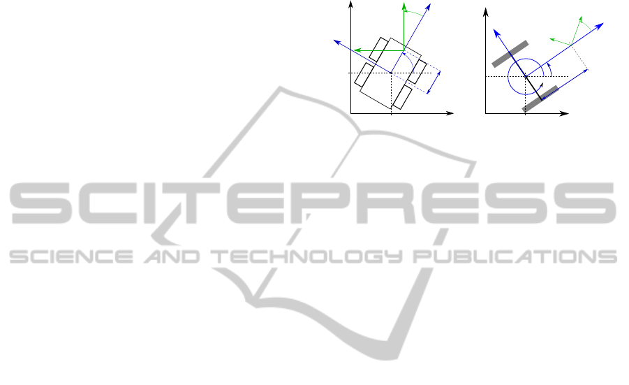
x
W
y
W
P
ref
v
θ
y
W
x
W
y
rob
x
rob
P
ref
y
cam
z
cam
θ
θ
cam
d
cam
ω
y
cam
z
cam
θ
cam
x
rob
d
cam
y
rob
y
x
Figure 1: Real Life Robot Model (left) vs Robot Reference
Kinematic Model(right).
2.2 Kinematic Model of the Robot
Let us consider Figure 1. The robot’s pose is defined
by vector (x,y,θ) where (x,y) and θ are respectively
its position and its orientation wrt the world frame
F
w
(O, ~x
w
, ~y
w
, ~z
w
). Furthermore, we propose another
frame F
rob
(P
re f
, ~x
rob
, ~y
rob
, ~z
rob
) attached to the robot
and yet a final frame F
cam
(C, ~x
cam
, ~y
cam
, ~z
cam
) at-
tached to the camera system. The angle between F
cam
and F
w
is θ
cam
and for this paper we will ignore the
tilt degree of freedom of the system. We consider a
non-holonomic 4-wheel skid-steering robot. Follow-
ing (Campion et al., 1996), provided that point P
re f
is chosen as a point on an imaginary axis that lies in
between both wheel axis, its kinematic model is given
by the following relations:
˙x(t)
˙y(t)
˙
θ(t)
˙
θ
cam
=
cos(θ(t)) 0 0
sin(θ(t)) 0 0
0 1 0
0 0 1
∗
ν(t)
ω(t)
ω
cam
(t)
(1)
where ˙q = [ν ω ω
cam
]
T
gathers the control inputs.
While ω and ω
cam
coincide with the angular veloci-
ties of the robot (about z
rob
) and camera (about x
cam
),
ν represents the linear velocity of the robot along its
axis x
rob
. From this result, we deduce the camera
kinematic screw wrt F
w
which is given by T
F
c
c
where
J is the robot’s Jacobian.
T
F
c
c
= J ˙q (2)
J =
−sin(θ
cam
) d
cam
∗ cos(θ
cam
) 0
cos(θ
cam
) d
cam
∗ sin(θ
cam
) 0
0 −1 −1
(3)
ICINCO2014-11thInternationalConferenceonInformaticsinControl,AutomationandRobotics
58
2.3 Visual Servoing
VS allows to control a robot using the information
provided by a camera (Chaumette and Hutchinson,
2006). Roughly speaking, it can be divided into two
main classes: 3D-VS, where the feature vector is pre-
sented in 3D and 2D-VS where the data used to con-
trol the robot is directly defined on visual cues. Since
it is less sensitive to noise than 3D-VS, we have used
the second kind of control. The goal is to make
the current visual signals s converge to their refer-
ence values s
∗
obtained at the desired (for the camera)
pose. To perform this task, we apply the VS technique
given in (Chaumette and Hutchinson, 2006) to mobile
robots as in (Pissard-Gibollet and Rives, 1995). The
proposed approach relies on the task function formal-
ism (Samson et al., 1991) and consists in expressing
the VS-task by the following task function to be reg-
ulated to zero:
e
V S
= s − s∗ (4)
In our case, the visual features s will be defined by a
target made of a set of N points of coordinates (X
i
,Y
i
)
in the image plane. By imposing an exponential de-
crease on e
V S
, a controller making e
V S
vanish is ob-
tained in (Chaumette and Hutchinson, 2006):
˙q =
ν
ω
ω
cam
= −λ ∗ ((L ∗ J)
−1
∗ e
V S
) (5)
where λ is a positive scalar or a positive definite ma-
trix and L represents the interaction matrix. This lat-
ter matrix allows to relate the variation of the visual
features in the image to the camera kinematic screw.
Hence it is crucial to compute ˙q. For one point L is
given by the following expression:
L =
0
X
i
z
i
X
i
Y
i
−1
z
i
Y
i
z
i
1 +Y
2
i
(6)
Here X
i
and Y
i
are the pixel coordinates in the camera
frame and z
i
represents the depth of this point i.
3 OBSTACLE AVOIDANCE
3.1 The Avoidance Strategy
As we have hinted in the introduction we strive to
achieve obstacle avoidance with the help of spirals. In
this paragraph, our work has been inspired by (Boy-
adzhiev, 1999) where the author has shown that the
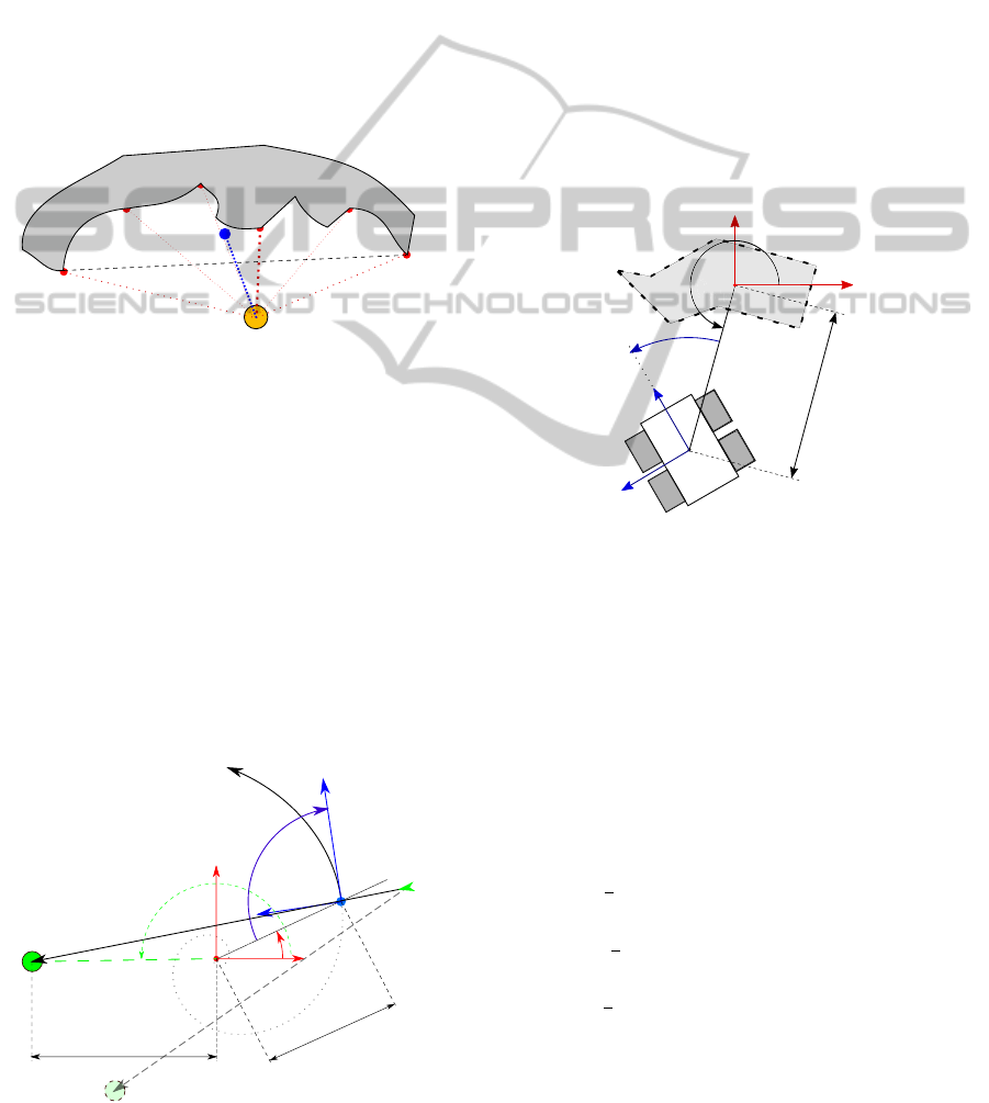
α
α
α
(a)
(b)
(c)
Figure 2: Three Schematics of Spiral Obstacle Avoidance
Patterns.
flight path of insects around a light source results in a
logarithmic spiral, also known as equiangular spiral.
Figure 2 gives a general idea of how this concept can
be applied for OA. Here we introduce three different
options (an outward, a circle and an inward spiral tra-
jectory) to circumvent a detected obstacle (gray poly-
gon) using the spiraling concept by choosing α
d
as
described on page 4. Before we get into more detail
on how to reach either a.), b.) or c.) let us take a step
back and look on how we define certain parameters
starting with the center point of the spiral.
3.2 Definition of the Spiral
3.2.1 Choosing the Spiral Center Point
To define the spiraling center point (SCP) we have
chosen to use the data provided by the LRF. Of this
data we will first define the obstacles face by search-
ing for adjacent points. To make this following tech-
nique work, we have to assume that adjacent points
belong to the same obstacle. Having detected the ob-
stacle our next step is to define its boundaries. We
will assume that the center point is located in be-
tween those boundaries and particularly in this paper
we will consider that the SCP is in the middle of both
outer boundaries of the obstacle. To choose the cen-
ter of the obstacle we will now take the middle of
both outer boundaries. Now we have the ”heading”
of the SCP, E
center
(see blue line in Figure 3). What
is still missing is the distance of this reference point
towards the robot. Therefore, the algorithm will sim-
ply choose the shortest distance towards the obstacle
from all LRF detected points (thickest red line). This
distance will then be projected along the previously
determined heading (blue line). To make sure that the
points we have branded as the obstacles outer bound-
aries are valid and to avoid outliners, the border of
ANavigationalFrameworkCombiningVisualServoingandSpiralObstacleAvoidanceTechniques
59
an obstacle must have adjacent points that are close
enough to justify the hypothesis that this point be-
longs to the obstacle. Furthermore, in order to choose
the closest distance to the obstacle the smallest LRF
values are examined with the help of a median filter.
Such an approach allows to benefit from nice robust-
ness properties, as our avoidance strategy relies on
several laser points as opposed to just one as it has
been done in all the previous works at hand (Folio
and Cadenat, 2005), (Adrien D. Petiteville and Cade-
nat, 2012).
The resulting point will be kept as the SCP for as long
as the robot is in a safe distance to the target. Should
it however, get too close to the obstacle, the SCP will
be recomputed with the newly collected LRF data.
x
E
center
Figure 3: Concept of estimating the Spiral Center Point.
3.2.2 Spiral Conventions and Definition
Once point E
center
has been defined and we attached
a frame denoted by F
E
(E
center
,~x
E
, ~y
E
,~z
E
) whose axes
are chosen to be equal to the ones of the world frame
F
w
(same orientation) we can start imagining an ap-
propriate OA. In Figure 4 we now present the spiral
concept and its conventions. A complete robot has
not yet been visualized in order to clarify our conven-
tions in a less overloaded figure.
First, we denote P
spiral
as one point of the spiral, while
T and N represent the tangent on the spiral and the
normal vector of it. The green arrow at the far right of
the figure indicates the previous heading of the robot
T
N
α
d
β
obs
x
E
y
E
r
d
P
target
A
P
target
B
r
target
β
target
E
center
P
spiral
Figure 4: Spiral Conventions.
and will be of importance for the sense of motion
which we will discuss later. The spiral we envision
is a equiangular spiral and defined by the following
polar equation in frame F
E
:
r
d
= r
0
∗ exp
cot(α
d
)∗(β
obs
0
−β
obs
)
(7)
where r
d
is the distance between E
center
and
P
spiral
, β
obs
represents the angle between x
E
and
~
E
center
P
spiral
. Furthermore α
d
is defined as the an-
gle from the connecting vector robot-obstacle and the
tangent to the spiral. Our convention is that the po-
sition of the robot at t = t
0
, the time when the OA is
first triggered, represents the first point of the spiral
and will therefore, determine r
0
, β
obs
and β
obs
0
. Of
those parameters only β
obs
will vary over time and r
0
and β
obs
0
will be set to the values of r
d
and β
obs
at
t = t
0
.
α
x
rob
x
obs
y
obs
P
ref
r
rob-obs
E
center
y
rob
β
obs
Figure 5: Parameters of the Robot Obstacle Relationship.
Now let us consider Figure 5 where we added a model
of the robot. In this figure, we denote r
rob−obs
as the
distance between points E
center
and P
re f
and α the an-
gle between~x
E
and
~
E
center
P
re f
. So in the optimal case
r
rob−obs
as well as α should be equal to their counter-
parts, r
d
and α
d
.
The equiangular spiral (from Equation 7) is defined
by four parameters r
0
, α
d
, β
obs
and β
obs
0
. So far we
managed to set all parameters but one. To properly
choose α
d
we may consider the following guidelines
deducted from (Boyadzhiev, 1999) (review Figure 2
on page 3):
• if α
d
>
π
2
: an outward spiral is performed and the
robot pulls away from the obstacle;
• if α
d
<
π
2
: an inward spiral is realized and the
robot closes the distance towards the obstacle;
• if α
d
=
π
2
: a circle is obtained and the robot main-
tains at a constant distance to the obstacle.
While the first and third cases seem to offer attractive
motion behaviors, the second one may also be inter-
esting if several obstacles lie in the robot’s vicinity
ICINCO2014-11thInternationalConferenceonInformaticsinControl,AutomationandRobotics
60

(e.g. a cluttered environment) or if a mobile obstacle
is expected to cross the vehicle path. Indeed, the robot
will then have the ability to go closer to the obstacle.
A nominal value for α
d
and its effects on the robot are
given in the results section.
3.2.3 Sense of Motion Around the Obstacle
One final detail we have not mentioned so far con-
cerns the sense of motion around the obstacle. In Fig-
ure 4 we have hinted on this ”orientation” of the spi-
ral which is dependent on the position of the target
(P
target
A
or P
target
B
) towards the robot and the obsta-
cle. In fact, when choosing our spiraling parameters
we have to decide on the orientation before. Taking a
look back onto the figure the robot has two options.
Either it moves clockwise, cw (e.g.: when P
target
B
is the target), or counter-clockwise, ccw (e.g.: when
P
target
A
is the target), around the obstacle. For now
there is only one condition which dictates our spiral
orientation will be the location of the target in rela-
tion to the robot reference (P
re f
) and the obstacle ref-
erence point (E
center
). P
target
B
, the green point with
an interrupted enclosing line displays a target which
would lead to a change in the spirals orientation to
a clockwise manner. For the situation mentioned be-
fore, where it would be necessary to recompute the
spiraling center point, we will keep the orientation to
avoid being trapped by the obstacle.
3.3 The Obstacle Avoidance Control
Law
3.3.1 Control of the Mobile Base
The intention of the following paragraph is to find a
control law which can be sent to the robot to make
it move according to the spiraling concepts presented
before. This control law was deduced from the anal-
ysis of the expected motion of the robot. First of all,
we have decided to impose a constant (non-zero) lin-
ear velocity denoted by ν
0
.
After that our approach for the control law is to firstly,
minimize the error between the desired angle (α
d
) and
the current angle of the robot towards the obstacle (α)
and secondly, to make the distance r
rob−obs
converge
towards r
d
given by Equation 7. The first assignment
is achieved by the first addend of ω (e
α
d
) in the man-
ner of a task function approach as it is used throughout
this paper (VS-controller and control of the camera
platform later on). Furthermore a parameter χ is intro-
duced which is dependent on the current distance be-
tween the obstacle and the robot, measured constantly
with the help of the LRF. Hence, χ will enable us to
address our second assignment for this control law.
Also, it resembles a precautionary measure which is
taken to ensure that the robot stays on the path we
envisioned and can never enter into dangerous areas
which in turn ensures a much smoother movement of
the robot. Since we have chosen to set the robot’s lin-
ear speed to a non-zero constant value ν
0
the angular
speed is the sole control input upon which we act to
guarantee the collision free navigation.
ω =
(
e
α
d
+ χ(r
d
), if ccw
−e
α
d
+ χ(r
d
), if cw
(8)
e
α
d
= α − α
d
(9)
Here χ is given in another task function approach:
χ =
(
e
r
d
∗ λ
r
, if ccw
−e
r
d
∗ λ
r
, if cw
(10)
e
r
d
= r
rob−obst
− r
d
(11)
where λ
r
is a positive gain and adjusts between our
angle and distance needs. We can furthermore ob-
serve that Equation 8 and Equation 10 are equipped
to deal with either a cw or a ccw motion arround the
obstacle. Equation 8 can be applied as long as the
sampling rate is sufficiently high and the differences
in the velocity of the robot and the obstacle do not ex-
ceed certain limits. Upon reaching those limits it is
still possible to compensate with the λ
r
. However, in
all simulations those limits were never reached.
3.3.2 Control of the Pan-Tilt-Unit
Following our previous paragraph, the mobile base is
controlled using the following velocities:
˙q
base
=
ν
0
ω
(12)
where ω is given by Equation 8. This control law en-
sures the non-collision. However, it is also necessary
to control the PTU, or simply pan-platform, of the
camera system so that the visual features are never
lost. This is a mandatory condition which insures that
it will be possible to switch back to VS, once the ob-
stacle will not be inducing any danger. Furthermore,
the continuous computation of VS is necessary for the
execution of the guarding conditions as we will see
soon. To do so, we propose to regulate the following
error to zero:
e
pan
= Y −Y
d
(13)
where Y and Y
d
corresponds to the current and desired
ordinate of the center of gravity of the target in the im-
age. Separating the terms related to the pan-platform
ANavigationalFrameworkCombiningVisualServoingandSpiralObstacleAvoidanceTechniques
61
and to the mobile base in the robot’s Jacobian leads
to:
T
c
= [J
b
J
pan
] ˙q (14)
Now introducing the interaction matrix L
y
corre-
sponding to the ordinate Y of a point, we may deduce
that:
˙
Y = L
y
T
c
= L
y
J
b
˙q
base
+ L
y
J
pan
ω
cam
(15)
A controller making e
pan
exponentially decrease to
zero is given by:
ω
cam
= −
1
L
y
J
pan
(λ
pan
e
pan
) + L
y
J
b
˙q
base
(16)
where λ
pan
is a positive scalar.
3.4 The Supervisor and its Guarding
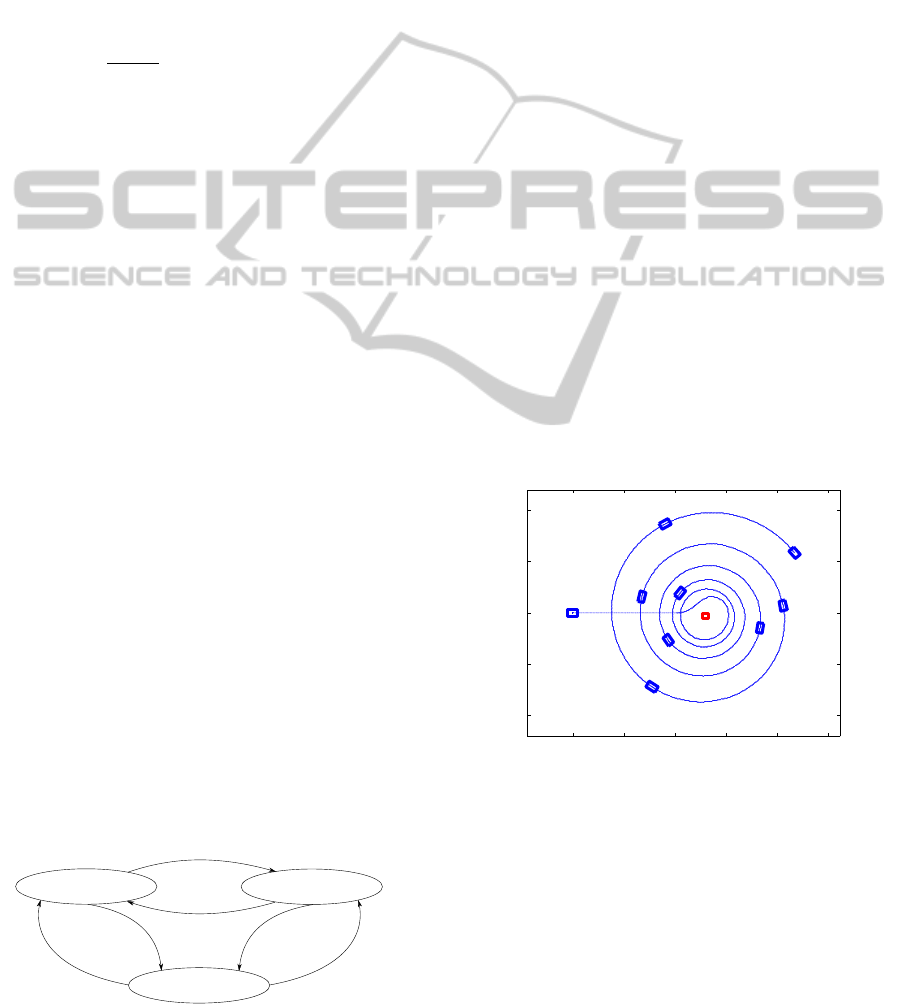
Conditions
The supervisor is the high-level-controller which is
able to choose from a list of controllers, such as VS
or OA, the most suitable controller for the situation at
hand. In Figure 6 a schematic can be found which ex-
plains how the supervisor is using guard conditions to
evaluate which controller is to be chosen. The ellipses
in this figure represent these different controllers and
the arrows visualize the possible switching directions.
A controller we have not talked about so far is the
”Trajectory based Navigation”. In cases where no
visual clues can be detected to guide the robot the
supervisor will switch to this controller to compute
the robot’s motion. The method used to do so is
presented in (Marder-Eppstein et al., 2010) and was
implemented in the Robot Operating System (ROS)
Navigation Stack. It relies on a constantly updated
metric map to guide the robot.
Guarding conditions, or simply guards, are methods
which tell the supervisor to switch behavior. Our
guard for switching to OA is very basic. Whenever
the LRF detects points which are closer than the trig-
ger distance (r
OA−trigger
), the supervisor will switch
to OA behavior. To disengage the OA when the ob-
stacle is passed we keep computing the VS controller
without applying its computed velocities to the robot
(Petiteville and Cadenat, 2014). Furthermore, we es-
timate the pose of the robot if we would apply these
Visual Servoing
Obstacle Avoidance
Trajectory based Navigation
(Path Planning)
VS-Error<Threshold
VS-Error>Threshold
r
rob-obs
<r
OA-trigger
r
rob-obs
>r
OA-trigger
r
rob-obs
>r
OA-trigger
r
rob-obs
<r
OA-trigger
Figure 6: Schematic of the Supervisor.
commands. This assessment is achieved with a simple
Euler Scheme (discretization) meaning we will com-
pute the next position of the robot by using its cur-
rent position and adding the derivative of the current
velocity. If the algorithm realizes that using the VS-
Controller will actually move the robot further away
from the obstacle, a guarding condition will instruct
the supervisor to switch back to VS. In order to not
constantly switch behaviors this situation needs to be
observed a certain number of times successively.
4 SIMULATION AND RESULTS
4.1 Simulation Environment
The Air-Cobot-Robot will be using ROS. Since the
recommended simulator for ROS is Gazebo we chose
this simulator as our test environment. However, in
order to visualize our findings we figured that nei-
ther ROS, Gazebo or even RVIZ can provide a suffi-
cient presentation of our findings in just a few images.
Thus, in order to present our simulation results we
used the ROS recording tool (ROS-bag) and a ground
truth Gazebo plug-in to capture the robot and obstacle
positions and orientation. Those recordings are then
read into Matlab and plotted as trajectories in a 2D-
plot. At ”http://homepages.laas.fr/mfutterl/” we pro-
vide a recording (video file) of the second experiment.
0 5 10 15 20 25
−10
−5
0
5
10
Position X in [m]
Position Y in [m]
Start
End
Figure 7: Proof of Concept of an outwards spiraling Obsta-
cle Avoidance.
Figure 7 displays one of those recordings. Here we
present our capability of spiraling around an obstacle
by applying Equations 8, 10 and 7 with an α
d
> 90
◦
.
The figure displays successive poses of a robot (blue
rectangles) going from left to right (blue path) and
also the static obstacle (red rectangle). As we can see,
the obstacle is successfully avoided by the robot exe-
cuting a spiral motion around it, as expected. Further-
ICINCO2014-11thInternationalConferenceonInformaticsinControl,AutomationandRobotics
62
more, one can observe that the performed spiral is an
outward spiral due to the chosen α
d
.
A
BC
D E F
T.1
T.3
T.4
T.2
C.2
C.3
−15 −10 −5 0 5 10 15 20 25 30
−15
−10
−5
0
5
10
15
Position X in [m]
Position Y in [m]
F.2
T.5
Figure 8: Simple Avoidance Experiment for static Obsta-
cles.
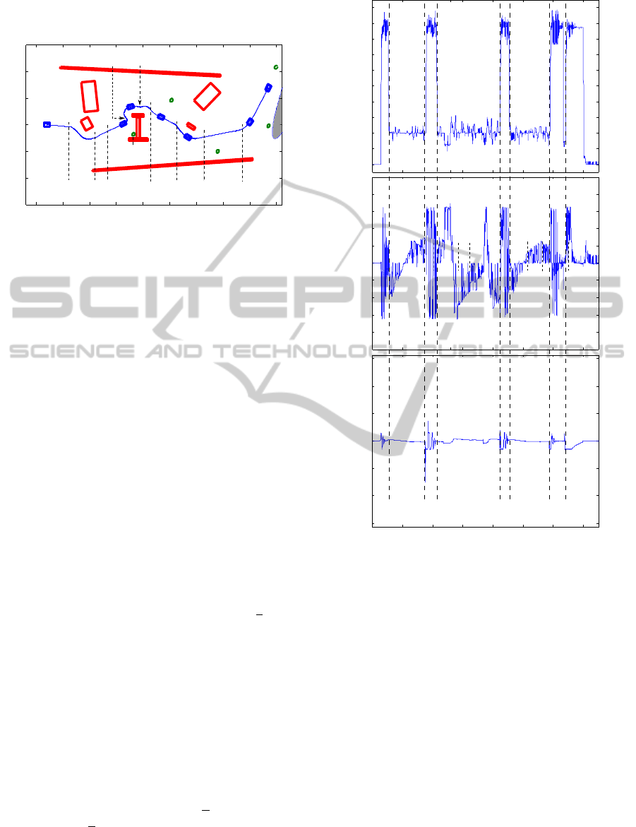
In Figure 8 we present a scenario where the OA con-
troller is coupled with a VS controller. The simulation
environment is set up with the projects requirements
in mind (provided video file). Mainly the approach
towards an aircraft (grey area on the far right side of
the figure) is simulated as well as reaching the first
checkpoint at its jet engine. All the obstacles (red
rectangles) are static and non-occluding and the dis-
tance at which the OA is triggered is set to 2.5 me-
ters. Furthermore, we have implemented a very basic
topological map allowing the robot to advance to the
next visual marker (T.1-T.5) whenever the VS error is
sufficiently low. Instead of spiraling around the obsta-
cle indefinitely, a guard enables the robot to leave the
OA controller when a safe passage towards the cur-
rent landmark is possible. By taking a closer look, we
can observe the VS behavior from Start to A, shortly
from B to C, from D to E and finally from F through
F.2 to the final position. The spiral obstacle avoid-
ance is used from A to B (counter-clockwise), from C
to D (cw) and from E to F (ccw) with an α
d
of
π
2
. Es-
pecially the second obstacle is interesting as it offers
the robot a convenient trap forcing it to recomputing
the spiral center point two times during its avoidance
(C.2 and C.3). For the other two obstacles, the re-
computation of the SCP is not necessary. By consult-
ing the results of this experiment we can conclude that
our approach is applicable and works as expected.
In Figure 9.top the linear velocity for the previous ex-
periment is presented. As before, the data is obtained
with the help of a Gazebo ground truth plug-in. We
can clearly see the time intervals in which the robot
was using the VS controller ('1.8
m
s
) and the OA
controller ('0.4
m
s
). The slight ”up and downs” dur-
ing the respective phases are due to the skid steering
drive controller and are matter of optimization at the
moment. The kinematic model of the robot forces it to
A
B C
DE F
0
0.2
0.4
0.6
0.8
1
1.2
1.4
1.6
1.8
2
Velocity in [m/s]
−1
−0.8
−0.6
−0.4
−0.2
0
0.2
0.4
0.6
0.8
1
Velocity in [rad/s]
0 1000 2000 3000 4000 5000 6000 7000
−3
−2
−1
0
1
2
3
Time in [s/100]
Positionin [rad]
F.2
Figure 9: Robot’s linear and angular Velocities and Camera
Angle.
slow down in order to apply higher changes in angu-
lar velocity. A better prediction of the obstacles shape
could make these higher angular changes irrelevant in
the future, thus, smoothing the robot’s trajectory. Fig-
ure 9.middle and .bottom give a view on the robot’s
angular velocity and the camera angle during the mis-
sion.
5 CONCLUSION
In this article we have shown that it is possible to use
the concepts found in (Boyadzhiev, 1999) and apply
them to the OA of a mobile robot. Furthermore, we
have succeeded in combining these techniques into a
navigational framework including a supervisor and a
VS controller. There are still some challenges which
ANavigationalFrameworkCombiningVisualServoingandSpiralObstacleAvoidanceTechniques
63

we have yet to conquer such as improving the tech-
niques to chose the center point of the Spiral (SCP)
from point-cloud data provided by the LRF. A more
sophisticated method to determine this point could be
found in either least square methods (also including a
window approach to remove points that are to old are
conceivable) or even in matching the acquired points
to a predefined simple shape (ellipsis, circle, rectan-
gle, etc.). At the moment we are working on applying
the algorithms shown in this paper onto moving ob-
stacles and also increasing the robustness of Equation
10 for those situations. Finally, as has been hinted on
before, smoothing the robot’s velocity controllers is
another subject we are currently working on. For the
future, we also plan to integrate presented concepts on
the real Air-Cobot-Robot and perform tests in a real
life situation.
REFERENCES
Adrien D. Petiteville, A. D. and Cadenat, V. (2012). From
the general navigation problem to its image based so-
lutions,. Workshop Vicomor. IROS 12. Portugal.
Boyadzhiev, K. N. (1999). Spirals and conchospirals in the
flight of insects. The College Mathematics Journal,
30(1):pp. 23–31.
Campion, G., Bastin, G., and Dandrea-Novel, B. (1996).
Structural properties and classification of kinematic
and dynamic models of wheeled mobile robots.
Robotics and Automation, IEEE Transactions on,
12(1):47–62.
Chaumette, F. and Hutchinson, S. (2006). Visual servo con-
trol. i. basic approaches. Robotics Automation Maga-
zine, IEEE, 13(4):82–90.
Cherubini, A., Grechanichenko, B., Spindler, F., and
Chaumette, F. (2013). Avoiding moving obstacles
during visual navigation. In Robotics and Automa-
tion (ICRA), 2013 IEEE International Conference on,
pages 3069–3074.
Cherubini, A., Spindler, F., and Chaumette, F. (2012). A
new tentacles-based technique for avoiding obstacles
during visual navigation. In Robotics and Automa-
tion (ICRA), 2012 IEEE International Conference on,
pages 4850–4855.
Damas, B. and Santos-Victor, J. (2009). Avoiding moving
obstacles: the forbidden velocity map. In Intelligent
Robots and Systems, 2009. IROS 2009. IEEE/RSJ In-
ternational Conference on, pages 4393–4398.
Folio, D. and Cadenat, V. (2005). A controller to avoid both
occlusions and obstacles during a vision-based navi-
gation task in a cluttered environment. In Decision
and Control, 2005 and 2005 European Control Con-
ference. CDC-ECC, pages 3898–3903.
Khatib, M. and Chatila, R. (1995). An extended potential
field approach for mobile robot sensor-based motions.
In Press, I., editor, Intelligent Autonomous Systems
(IAS), pages 490–496, Karlsruhe, Germany.
Koenig, S. and Likhachev, M. (2005). Fast replanning for
navigation in unknown terrain. Robotics, IEEE Trans-
actions on, 21(3):354–363.
Lamiraux, F., Bonnafous, D., and Lefebvre, O. (2004).
Reactive path deformation for nonholonomic mobile
robots. Robotics, IEEE Transactions on, 20(6):967–
977.
Marder-Eppstein, E., Berger, E., Foote, T., Gerkey, B.,
and Konolige, K. (2010). The office marathon: Ro-
bust navigation in an indoor office environment. In
Robotics and Automation (ICRA), 2010 IEEE Inter-
national Conference on, pages 300–307.
Matsumoto, Y., Inaba, M., and Inoue, H. (1996). Vi-
sual navigation using view-sequenced route represen-
tation. In Robotics and Automation, 1996. Proceed-
ings., 1996 IEEE International Conference on, vol-
ume 1, pages 83–88 vol.1.
Mcfadyen, A., Corke, P., and Mejias, L. (2012a). Rotor-
craft collision avoidance using spherical image-based
visual servoing and single point features. In Intelligent
Robots and Systems (IROS), 2012 IEEE/RSJ Interna-
tional Conference on, pages 1199–1205.
Mcfadyen, A., Mejias, L., and Corke, P. (2012b). Visual
servoing approach to collision avoidance for aircraft.
In 28th Congress of the International Council of the
Aeronautical Sciences 2012, Brisbane Convention &
Exhibition Centre, Brisbane, QLD.
Owen, E. and Montano, L. (2005). Motion planning in dy-
namic environments using the velocity space. In Intel-
ligent Robots and Systems, 2005. (IROS 2005). 2005
IEEE/RSJ International Conference on, pages 2833–
2838.
Petiteville, A. D. and Cadenat, V. (2014). An anticipative
reactive control strategy to deal with unforeseen ob-
stacles during a multi-sensor-based. ECC.
Pissard-Gibollet, R. and Rives, P. (1995). Applying visual
servoing techniques to control a mobile hand-eye sys-
tem. In Robotics and Automation, 1995. Proceedings.,
1995 IEEE International Conference on, volume 1,
pages 166–171 vol.1.
Samson, C., Espiau, B., and Borgne, M. L. (1991). Robot
Control: The Task Function Approach. Oxford Uni-
versity Press.
Ulrich, I. and Borenstein, J. (2000). Vfh*: local obstacle
avoidance with look-ahead verification. In Robotics
and Automation, 2000. Proceedings. ICRA ’00. IEEE
International Conference on, volume 3, pages 2505–
2511 vol.3.
Vilca, J., Adouane, L., and Mezouar, Y. (2013). Reactive
navigation of a mobile robot using elliptic trajecto-
ries and effective online obstacle detection. Gyroscopy
and Navigation, 4(1):14–25.
ICINCO2014-11thInternationalConferenceonInformaticsinControl,AutomationandRobotics
64
