
Artificial Neural Network Models of Intersegmental Reflexes
Alicia Costalago Meruelo
1
, David M. Simpson
1
, S. Veres
2
and Philip L. Newland
3
1
Faculty of Engineering and the Environment, University of Southampton, Southampton, U.K.
2
Department of Automatic Control and Systems Engineering, University of Sheffield, Sheffield, U.K.
3
Centre for Biological Sciences, University of Southampton, Southampton, U.K.
Keywords: Reflex, Artificial Neural Network, ANNs, Time Delay Neural Network, Metaheuristic Algorithm,
Evolutionary Programming, Particle Swarm Optimisation, Chordotonal Organ, Locust.
Abstract: In many animals intersegmental reflexes are important for postural control and movement making them
ideal candidates for the bio-inspired design of medical treatment for neuromuscular injuries in cases such as
drop foot and possibly in robot design. In this paper we study an intersegmental reflex of the foot (tarsus) of
the locust hind leg, which is a reflex that raises the tarsus when the tibia is flexed and depresses it when the
tibia is extended. A novel method is described to quantify the intersegmental responses in which an
Artificial Neural Network, the Time Delay Neural Network, is applied. The architecture of the network is
optimised through a metaheuristic algorithm to produce accurate predictions with short computational time
and complexity and high generalisation to different individual responses. The results show that ANNs
provide accurate predictions when trained with an average reflex response to Gaussian White Noise
stimulation compared to autoregressive models. Furthermore, the network model can calculate the
individual responses from each of the animals and responses to another input such as a sinusoid. A detailed
understanding of such a reflex response could be included in the design of orthoses or functional electrical
stimulation treatments to improve walking in patients with neuromuscular disorders.
1 INTRODUCTION
Intersegmental reflexes are key elements in postural
control and locomotion in many animals. One of
their roles is to provide stability and agility to
movements (Prochazka, Clarac et al. 2000). A reflex
response is a neurally mediated reproducible
movement graded with respect to stimulus intensity
that is not controlled voluntarily. Understanding
such types of reflexes might improve current
medical treatments for neuromuscular injuries such
as drop foot. It can also be applied to the design of
prosthesis or active prosthesis for amputees (Herr
and Grabowski 2011).
Intersegmental reflexes have been observed in
many vertebrates and invertebrates, such as cats,
crustaceans and insects (Burrows and Horridge
1974, Bush, Vedel et al. 1978, Field and Rind 1981,
Smith, Hoy et al. 1985). Vertebrates and
invertebrates have many similarities in motor control
(Pearson 1993) and by studying intersegmental
reflexes in insects, the complexity of the motor
system and reflex responses is reduced, aiding its
understanding. In locusts, the tarsus is moved by
only three motor neurons (Burrows 1996). The tarsal
intersegmental reflex elevates the tarsus when the
tibia is extended and depresses it when the tibia is
flexed (Figure 1). The response is therefore initiated
by knee joint kinetics, which are monitored by a
sensory organ in the femur, the femoral chordotonal
organ (FeCO).
Figure 1: Tarsal intersegmental reflex when the tibia is
fully flexed, in 60° and fully extended.
The chordotonal organ is connected to the tibia
by a strand, an apodeme, which pulls on the FCO
when the tibia is flexed and reduces the tension on
the FCO when the tibia is extended (Shelton,
Stepehn et al. 1992, Field and Matheson 1998).
Mathematical models have been used for many
years to understand and describe similar reflexes.
Linear and nonlinear models, such as Wiener
24
Costalago Meruelo A., M. Simpson D., Veres S. and L. Newland P..
Artificial Neural Network Models of Intersegmental Reflexes.
DOI: 10.5220/0005029000240031
In Proceedings of the International Conference on Neural Computation Theory and Applications (NCTA-2014), pages 24-31
ISBN: 978-989-758-054-3
Copyright
c
2014 SCITEPRESS (Science and Technology Publications, Lda.)
methods, have been used in many studies (Newland
and Kondoh 1997, Dewhirst, Simpson et al. 2009).
Although these methods provide a quantitative
description of the dynamic transfer characteristics of
the system, they can contain different types of
estimation errors (Korenberg and Hunter 1990).
Artificial Neural Networks (ANNs) are considered
to be able to approximate any continuous function
(Haykin 1999), including non-linear systems (Hunt,
Sbarbaro et al. 1992), they can adapt and generalise
better than other mathematical methods (Benardos
and Vosniakos 2007) and can be easily implemented
in software and hardware devices (Hunt, Sbarbaro et
al. 1992, Twickel, Büschges et al. 2011). Another
issue is that, to date, mathematical models of
biological systems have only been fitted to
individual responses, i.e. the parameters are fitted to
the response of one individual, which can be a poor
representation of a population (Marder and Taylor
2011).
This paper describes novel methods to quantify
intersegmental responses in the locust hind leg
tarsus, describes a new mathematical approach to
model and predict the tarsal reflexes using ANNs
and asks whether individual responses or the average
response should be used to model and study the
system.
2 METHODS
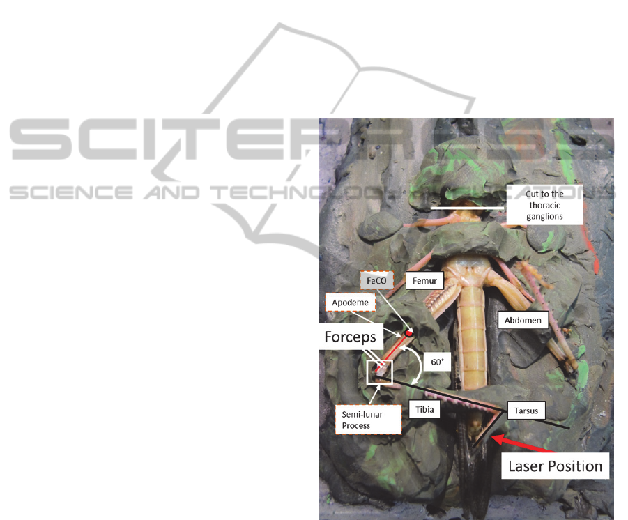
2.1 Experimental Methods
Adult male and female locusts (Schistocerca
gregaria) were fixed in modelling clay ventral side
up, with the femur fixed at 60° from the abdomen
and with the tibia fixed at an angle of 60° to the
femur, an angle which represents the middle of the
linear range movement of the FeCO apodeme
(Figure 2). The FeCO was exposed by removing a
small piece of cuticle at the distal end of the femur,
and the cavity was perfused with locust saline. The
FeCO apodeme was grasped with a pair of fine
forceps tip attached to a shaker (permanent magnet
shaker LDS V101). The shaker was driven by a
signal generated in Matlab
®
, which was amplified
and converted to analogue via a digital-to-analogue
(DA) converter (USB 2527 data acquisition card
(DAC), Measure Computing Norton, MA, USA).
The movement response in the locust tarsus was
recorded with a Keyence laser displacement sensor
(LK G3001V controller, LK G32 Head, Keyence)
aimed at the last segment of the tarsus.
The stimulus signals were designed and applied
through Matlab
®
. Locusts walk at a step frequency
of approximately 3 Hz (Burrows and Horridge 1974)
and for this reason, Gaussian White Noise (GWN)
was produced band-limited between 0 - 5 Hz, and a
sinusoidal input simulating walking was applied at 1
Hz. GWN was chosen since it contains all the
frequencies within that band and all the amplitudes
within a range. The maximum peak-to-peak
amplitude of the input signals was approximately 1
mm, which represents a femoro-tibial displacement
of 90° (Field and Burrows 1982, Dewhirst, Angarita-
Jaimes et al. 2012). The signals were scaled so that
approximately 99.7 % of their values fall in the
femoro-tibial joint angle between 20° and 100° (0.9
mm of displacement of the FeCO apodeme). The
frequency and phase response of the equiment was
linear between 0 and 200 Hz.
Figure 2: Image of a locust showing the set up for
analysis. The forceps were attached to the apodeme in the
distal part of the femur and a laser was aimed at the tarsus
to monitor its movements.
2.2 Mathematical Methods
2.2.1 Data Post-Processing
Recordings of tarsal movement from eight locusts
were made following the procedure described and
recorded at a sampling frequency of 10,000 Hz. The
ArtificialNeuralNetworkModelsofIntersegmentalReflexes
25
mean value was subtracted from the recordings to
eliminate any effect of laser position. To eliminate
low frequency noise and spontaneous movements
not related to the applied stimulus a third order high-
pass Butterworth filter was applied with a cut off
frequency of 0.2 Hz. The data was then resampled to
500 Hz after applying an anti-alias filter, a third
order Butterworth with cut off frequency of 200 Hz,
thereby reducing file size and processing time. Both
Butterworth filters were applied in the forward and
reverse directions to avoid introducing any phase
delay. An average reflex response was calculated
using the responses from the eight individuals to test
whether the average is representative of the system
or is if it is better to use individual responses
2.2.2 Artificial Neural Networks
To model the intersegmental reflex responses of the
tarsus a dynamical artificial neural network is
proposed, a Time Delay Neural Network (TDNN)
(Waibel, Hanazawa et al. 1989). This network uses
delayed versions of the input to estimate the output,
turning the static Feed-Forward Network into a
dynamic network (Haykin 1999). Using this, we
assumed the reflex responses to be a combination of
current and past input samples. The network is
formed by an input node, an output node, and a
number of hidden layers and with hidden nodes. The
activation function for each hidden node is the
sigmoid. The output node has a linear function, so
all the non-linear calculations are performed inside
the network. The training algorithm for the network
is the Levenberg - Marquadt back-propagation
algorithm, that has higher accuracy and faster
convergence time compared to classical back-
propagation algorithms (Bishop 1995). The number
of delayed samples used in the input is set to 100
samples, which is based on preliminary work
(optimisation of decrease in NMSE as the delay
increases for a set architecture). The architecture of
the network is optimised using a metaheuristic
algorithm presented in the next section.
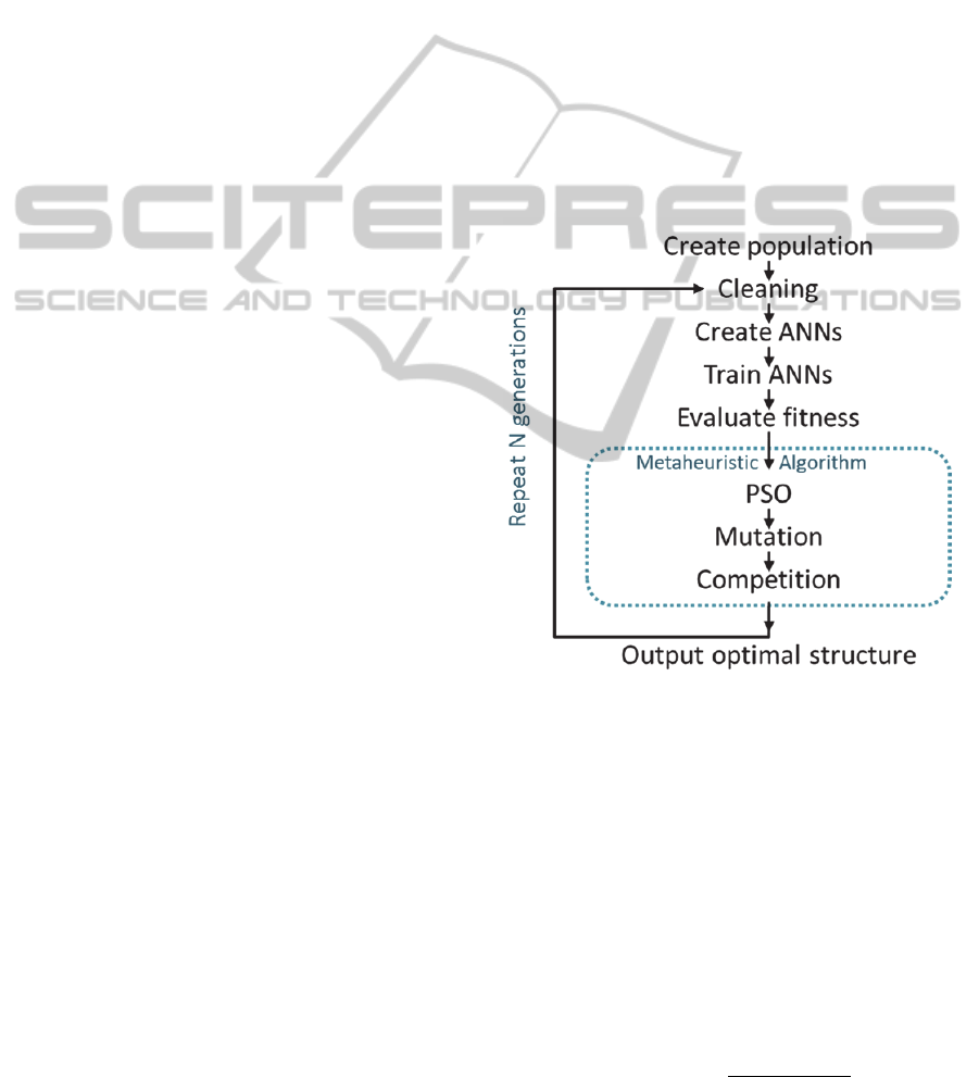
2.2.3 Metaheuristic Algorithm
The choice of the architecture of a neural network
affects the performance of such network. In this
case, the optimal networks should have high
accuracy and low complexity to reduce
computational time, and should be able to
generalise, i.e. it should not over-fit the training
data. To choose a performance optimal for the task
an algorithm is proposed (Figure 3) based on a
combination of Evolutionary Programming and
Particle Swarm Optimisation (PSO) (Kennedy and
Eberhart 1995, Eiben and Smith 2003). Similar
algorithms have been successfully applied
previously to design artificial neural network
architectures (Benardos and Vosniakos 2007,
Suraweera and Ranasinghe 2008). The algorithm
creates a population of possible TDNN solutions,
composed of random individuals. Each individual
denotes the architecture of a neural network in a
vector representation, with architectures limited to 5
hidden layers and 32 nodes per layer (Carvalho,
Ramos et al. 2011), which provide a wide range to
determine the optimal architecture. An individual
has the form:
(1)
Where η is the individual or candidate TDNN
architecture, and n
i
the number of nodes in the layer
i.
Figure 3: Metaheuristic algorithm for the design of the
TDNN architecture.
A cleaning function is applied to the population
of randomly initiated individuals η
j
, so that no
network contains 0 hidden layers. Subsequently, the
networks are created and trained with two thirds of
the GWN average response calculated across
individuals. The networks are then tested with the
third GWN not used on the training and their
performance and fitness is evaluated. The
performance is calculated as the Normalised Mean
Square Error (NMSE) between the predicted output
and the recorded output
.
%
100 ∙
∑
2
1
∑
2
1
(2)
NCTA2014-InternationalConferenceonNeuralComputationTheoryandApplications
26

The fitness function designed (Equation 3) evaluates
the performance of the network, its size, and
indirectly, the computational time. Since the
networks are set to train for a limited amount of
iterations, poor performance is obtained if they are
not fully trained by then.
100
%
∙
∑
(3)
Where is a constant set to 0.002 (based on
preliminary trial an error experiments) and
∑
is the
number of nodes in the network.
The fitness
evaluates the accuracy of the network and uses a
penalty factor dependant on the network size. Using
the fitness function, the architectures are modified
using PSO and mutation. PSO uses a population
approach where all individuals work together in the
search space to find the optimum. The mutation rate
adds random jumps in the search space to avoid
local maxima. For PSO the architecture of the
network represents its “position”,
. Its
“velocity”,
, is the difference between the
actual position and its previous position.
1
∙
2∙
∙
2∙
∙
(4a)
1
1
(4b)
Where 1.05 is the inertia weight (Shi and
Eberhart 1998),
and
are random numbers that
evaluate the contribution from the personal best of
the individual
and the global best of the
population
over the generations. The mutation
algorithm uses a dynamical mutation rate
(Equation 5) like the one used by Angeline,
Saunders et al. (1994).
1
(5)
Where is the fitness of an individual and
is the fitness of the best performing
individual. The mutation rate is larger if the network
is performing poorly and smaller if the fitness is
high, fine tuning in the optimal architecture. Once
the individuals have been modified, a competition
algorithm ensures that the fittest of the pair parent-
offspring passes to the next generation.
The algorithm is repeated over a number of
generations, in this particular case for 50
generations, or until an optimal network is found.
2.2.4 Autoregressive Model
To compare the results of the TDNN, an auto-
regressive (AR) model of the tarsal movements is
developed. As with the TDNN, the model assumes
that the tarsal response is a combination of current
and past input samples. Considering the discrete
form, the response of the system can be
characterised as:
∙
(6)
Where
is the response,
is the transfer
function of the system,
is the stimulus and
is the noise. To calculate de parameters of
the least square method is used. The equation of the
Minimum Mean Square Error cost function (Haykin
2002) is rearranged and it is assumed that the
prediction is a linear function of the impulse
response function. Combining the cost function with
the system response, the least square estimate of the
AR parameters is:
(7)
Where is the output, is the pre-windowed
matrix (Ljung 1999) and
the estimated model
parameters. For a full derivation see Dewhirst
(2013).
To compare the results from both mathematical
models, the NMSE (Equation 2) is going to be used,
when the model is tested with the same data not used
in training.
3 RESULTS
3.1 Intersegmental Reflex Responses
The movements of the tarsus recorded and post-
processed show that as the tibia is extended the
tarsus is depressed and when the tibia flexes the
tarsus is levated (Figure 4) which corroborates the
Figure 4: Tarsal intersegmental average response recorded
with shaker stimulus applied for the input at 1 Hz.
ArtificialNeuralNetworkModelsofIntersegmentalReflexes
27
results described by Burrows and Horridge (1974).
There is also an observable delay between the input
to the FCO and the response in the tarsus of 0.1 s,
resulting from known neural conduction times and
synaptic delays (Burrows, 1996).
3.2 Metaheuristic Algorithm TDNN
Architecture
Using the responses from the eight animals and the
average response to band-limited GWN the
algorithm was run until the optimal architectures for
each response were obtained (Table 1), a total of 9
models. While the algorithm was set to a maximum
of five layers and 32 nodes per layer, the optimal
architectures are limited to two layers and a
maximum of five nodes per layer. The algorithm
was set to run over 50 iterations or generations,
however, the ANN architectures converge and the
best or optimal network was obtained after the 35
th
generation for all the individual responses, including
the average response. Therefore, we can assume it
has reached the maximum fitness within 35
generations.
Table 1: Number of nodes per layer for the TDNN
designed using the metaheuristic algorithm.
Layer 1 Layer 2
Average response 4 -
Animal 1 3 -
Animal 2 5 -
Animal 3 5 1
Animal 4 2 1
Animal 5 3 1
Animal 6 3 -
Animal 7 4 -
Animal 8 3 -
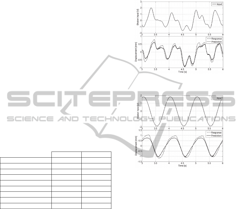
3.3 TDNN and AR Performance of the
Average Response
The TDNN and AR optimised for the average
response across animals were tested using unseen
GWN data and a sinusoidal input not used in the
training or the algorithm. The TDNN was able to
predict the averaged responses to both stimuli with a
high accuracy. The NMSE (%) between the
predicted response and the average GWN response
recorded was 13.85 % for the TDNN (Figure 4) and
27.18 % for the AR model. This same network was
tested with a 1 Hz input to study its generalisation to
a different input (Figure 5). The performance of the
network with the 1 Hz data is NMSE = 4.3 %, while
the AR model was 4.6 %, suggesting that both
models were able to generalise to at least one other
input when trained with GWN.
Figure 5: Prediction of the TDNN of the average reflex
response to a GWN stimulus. The NMSE = 13.85 %.
Figure 6: Prediction of the TDNN of the average reflex
response to a 1 Hz stimulus, with NMSE = 4.3 %.
3.4 TDNN and AR Performance of the
Individual Responses
The models designed for the individual responses,
TDNNs and AR models, were also tested with
unseen data, both from GWN and 1 Hz sinusoidal
stimulation to the FCO. This section studies the
accuracy of the models trained with GWN responses
from an individual and tested with responses from
the same individual as training, but not the same
data. The mean NMSE for all the TDNN with GWN
was µ = 26.1 % (standard deviation σ = 9.2) (Table
2), where some of the models perform better than
others. In the case of the AR models, the mean was
µ = 53.5 % (standard deviation σ = 21.7). When
tested with 1 Hz sinusoids, some of the TDNN
performed poorly (µ = 97.5 %, σ = 128.9, due to two
NMSE higher than 100 %), while others had low
prediction errors. In the case of the AR models, the
predictions were better on average (µ = 43.8 %, σ =
41.1), with only one with a high error. A statistical
NCTA2014-InternationalConferenceonNeuralComputationTheoryandApplications
28

analysis was performed to compare the TDNN and
the AR models. The results show that, when tested
with GWN, they are statistically different (t(7) = -
3.02, p = 0.009), however, with a 1 Hz sinusoid
although there is a large difference in the mean
values, the models are not significantly different
(t(7) = 1.14, p = 0.14).
Visual inspection of the poor performance of the
models with some of the 1 Hz responses shows that
the models overestimate the amplitude of the actual
response. Such differences in amplitude are due to
measurement noise, variability across individuals,
and the motor neuron responses to a stimulus
(Schneidman, Brenner et al. 2000, Marder and
Taylor 2011). These results emphasized the
differences across individual responses and the
problems of choosing only one individual to model a
system and use this as a generic model for all
animals.
Table 2: NMSE of the individual models when tested with
unseen GWN and 1 Hz sinusoidal inputs from the same
individual as training, but not the same response as used in
the training.
TDNN AR
GWN 1 Hz GWN 1 Hz
Animal 1 15.4 10.9 27.2 4.6
Animal 2 28.6 11.0 81.3 11.8
Animal 3 20.8 > 100 41.5 13.0
Animal 4 17.1 26.8 49.9 80.4
Animal 5 28.0 55.9 71.1 61.4
Animal 6 28.7 99.5 82.6 33.2
Animal 7 39.5 20.0 38.2 <100
Animal 8 42.7 > 100 33.9 13.7
Mean 26.1 97.5 53.5 43.8
3.5 Performance of the Average
Response TDNN and AR Models
with Individual Responses
We then analysed the accuracy of the TDNN and the
AR models trained with the average response when
predicting individual responses to GWN and 1 Hz
inputs, and evaluate if the average response is
representative of the population.
The NMSE values obtained for the TDNN
showed that the network trained with the average
response is able to predict responses in all
individuals to GWN (µ = 34.5 %, σ = 7.0) and to 1
Hz sinusoid, with the exception of Animal 3 and 6
(µ = 45.1 %, σ = 56.0). The AR model has poorer
performance with GWN (µ = 70.8 %, σ = 53.9),
although its performance is similar with 1 Hz (µ =
43.8 %, σ = 41.1), including the poor performance
with the same individuals. The TDNN provides a
significantly better performance than the AR model
for GWN inputs (t(7) = -2.08, p = 0.03), however,
for 1 Hz inputs, they are not significantly different
(t(7) = 0.15, p = 0.44).
The differences between the NMSE of the
individual TDNNs and the NMSE of the TDNN
trained with the average response and tested with the
individuals are not significantly different (t(7) = 1.4,
p = 0.2), suggesting that the TDNN trained with the
average response across the eight individuals is a
good representation of the system.
Table 3: NMSE of the TDNN trained with the average
response when predicting individual responses to GWN
and 1 Hz inputs.
TDNN AR
GWN 1 Hz GWN 1 Hz
Animal 1
34.4 7.7 >100 11.8
Animal 2
27.3 14.1 41.5 13.0
Animal 3
34.1 > 100 55.7 80.4
Animal 4
36.7 12.7 65.0 61.4
Animal 5
46.5 33.4 >100 33.2
Animal 6
34.6 > 100 32.8 >100
Animal 7
38.6 19.3 35.3 13.7
Animal 8
23.4 9.0 29.8 13.5
Mean
34.5 45.1 70.8 43.8
4 CONCLUSIONS
The methods described here were used to model the
reflex responses of the tarsus of the hind leg of the
locust. The intersegmental reflex responses recorded
were similar to those described by Burrows and
Horridge (1974): raising the foot when the tibia was
flexed and lowering the foot when the tibia was
extended, matching the natural movement of the foot
when walking in locusts and humans. Such
movement has been speculated to be related to
postural stability and agility (Burrows, Laurent et al.
1988, Büschges 2005).
The results have also shown that such responses
can be modelled using AR models and optimised
ANNs. The metaheuristic algorithm developed was
able to find an optimal and relatively parsimonious
network based on the specifications given. The
combination of PSO and dynamic mutation provided
a fast convergence in the design of ANNs, although
the data cannot be directly compared to other
publications, since, based on the authors knowledge,
no similar modelling has been done.
ArtificialNeuralNetworkModelsofIntersegmentalReflexes
29

The TDNN optimised and trained with the responses
to band-limited GWN predicts the responses
accurately for unseen band-limited GWN and
sinusoidal inputs, significantly better than the AR
model in the case of GWN stimuli. Furthermore, the
TDNN trained with the average response is also able
to predict responses in different individuals,
although with limited accuracy. The accuracy of the
average response TDNN model was not statistically
different to that of the individual models, which
suggests that, in this case, the average response is a
good representation of the system. Furthermore, the
NMSE values are similar to those obtained with
Wiener methods in locusts electrophysiological
responses of tibial motor neurons (Dewhirst,
Simpson et al. 2009), which suggests that ANNs
could be a good approach to model nervous systems.
The errors in the predictions are related to the
levels of measurement noise, background
spontaneous activity and individual differences in
the responses (Schneidman, Brenner et al. 2000,
Faisal, Selen et al. 2008, Marder and Taylor 2011).
There is, however, an underlying response common
to all individuals that the TDNN is able to model
and predict accurately, but the noise and the inherent
response from each animal cannot be predicted with
a generic model.
Therefore, the TDNN model of the average
reflex response exceeds the performance of the AR
model and is a good candidate model to be
considered towards the understanding of nervous
systems and motor control. It could also be used in
the design of treatment for neuromuscular injuries,
such as drop foot. Similar reflexes could also be
applied in the design of active prosthesis or
autonomous robots.
ACKNOWLEDGEMENTS
Alicia Costalago Meruelo was supported by a
studentship from The Institute for Complex Systems
Simulation (ICSS), funded by the Engineering and
Physical Sciences Research Council (UK) and the
University of Southampton.
REFERENCES
Angeline, P. J., G. M. Saunders and J. B. Pollack (1994).
"An evolutionary algorithm that constructs recurrent
neural networks." Neural Networks, IEEE
Transactions on 5(1): 54-65.
Benardos, P. G. and G.-C. Vosniakos (2007). "Optimizing
feedforward artificial neural network architecture."
Eng. Appl. Artif. Intell. 20(3): 365-382.
Bishop, C. M. (1995). Neural networks for pattern
recognition, Oxford university press.
Burrows, M. (1996). The neurobiology of an insect brain.
Oxford University Press, Oxford ;.
Burrows, M. and G. A. Horridge (1974). "The
Organization of Inputs to Motoneurons of the Locust
Metathoracic Leg." Philosophical Transactions of the
Royal Society of London. Series B, Biological Sciences
269(896): 49-94.
Burrows, M., G. J. Laurent and L. H. Field (1988).
"Proprioceptive inputs to nonspiking local
interneurons contribute to local reflexes of a locust
hindleg." The Journal of Neuroscience 8(8): 3085-
3093.
Büschges, A. (2005). "Sensory Control and Organization
of Neural Networks Mediating Coordination of
Multisegmental Organs for Locomotion." Journal of
Neurophysiology 93(3): 1127-1135.
Bush, B. M., J. P. Vedel and F. Clarac (1978).
"Intersegmental reflex actions from a joint sensory
organ (CB) to a muscle receptor (MCO) in decapod
crustacean limbs." The Journal of Experimental
Biology 73(1): 47-63.
Carvalho, A. R., F. M. Ramos and A. A. Chaves (2011).
"Metaheuristics for the feedforward artificial neural
network (ANN) architecture optimization problem."
Neural Comput. Appl. 20(8): 1273-1284.
Dewhirst, O. P. (2013). Validation of Nonlinear System
Identification Models of the Locust Hind Limb
Control System using Natural Stimulation. PhD
Thesis, Southampton University.
Dewhirst, O. P., N. Angarita-Jaimes, D. M. Simpson, R.
Allen and P. L. Newland (2012). "A system
identification analysis of neural adaptation dynamics
and nonlinear responses in the local reflex control of
locust hind limbs." J Comput Neurosci: 1-20.
Dewhirst, O. P., D. M. Simpson, R. Allen and P. L.
Newland (2009). Neuromuscular reflex control of limb
movement - validating models of the locusts hind leg
control system using physiological input signals.
Neural Engineering, 2009. NER '09. 4th International
IEEE/EMBS Conference.
Eiben, A. E. and J. E. Smith (2003). Introduction to
Evolutionary Computing, SpringerVerlag.
Faisal, A. A., L. P. J. Selen and D. M. Wolpert (2008).
"Noise in the nervous system." Nat Rev Neurosci 9(4):
292-303.
Field, L. H. and M. Burrows (1982). "Reflex Effects of the
Femoral Chordotonal Organ Upon Leg Motor
Neurones of the Locust." Journal of Experimental
Biology 101(1): 265-285.
Field, L. H. and T. Matheson (1998). Chordotonal Organs
of Insects. Advances in Insect Physiology. P. D.
Evans, Academic Press. Volume 27: 1-228.
Field, L. H. and F. C. Rind (1981). "A single insect
chordotonal organ mediates inter- and intra-segmental
NCTA2014-InternationalConferenceonNeuralComputationTheoryandApplications
30

leg reflexes." Comparative Biochemistry and
Physiology Part A: Physiology 68(1): 99-102.
Haykin, S. (1999). Neural networks: a comprehensive
foundation, Prentice Hall PTR.
Haykin, S. S. (2002). Adaptive filter theory, Prentice Hall.
Herr , H. M. and A. M. Grabowski (2011). "Bionic ankle–
foot prosthesis normalizes walking gait for persons
with leg amputation." Proceedings of the Royal
Society B: Biological Sciences.
Hunt, K. J., D. Sbarbaro, R. Żbikowski and P. J. Gawthrop
(1992). "Neural networks for control systems—A
survey." Automatica 28(6): 1083-1112.
Kennedy, J. and R. Eberhart (1995). Particle swarm
optimization. Neural Networks, 1995. Proceedings.,
IEEE International Conference.
Korenberg, M. and I. Hunter (1990). "The identification of
nonlinear biological systems: Wiener kernel
approaches." Annals of Biomedical Engineering 18(6):
629-654.
Ljung, L. (1999). System Identification. Wiley
Encyclopedia of Electrical and Electronics
Engineering, John Wiley & Sons, Inc.
Marder, E. and A. L. Taylor (2011). "Multiple models to
capture the variability in biological neurons and
networks." Nat Neurosci 14(2): 133-138.
Newland, P. L. and Y. Kondoh (1997). "Dynamics of
Neurons Controlling Movements of a Locust Hind Leg
III. Extensor Tibiae Motor Neurons." Journal of
Neurophysiology 77(6): 3297-3310.
Pearson, K. G. (1993). "Common principles of motor
control in vertebrates and invertebrates." Annual
review of neuroscience 16(1): 265-297.
Prochazka, A., F. Clarac, G. E. Loeb, J. C. Rothwell and J.
R. Wolpaw (2000). "What do reflex and voluntary
mean? Modern views on an ancient debate."
Experimental Brain Research 130(4): 417-432.
Shelton, P. M. J., R. O. Stepehn, J. J. A. Scott and A. R.
Tindall (1992). "The Apodeme Complex Of The
Femoral Chordotonal Organ In The Metathoracic Leg
Of The Locust Schistocerca Gregaria." Journal of
Experimental Biology 163(1): 345-358.
Shi, Y. and R. C. Eberhart (1998). A modified particle
swarm optimizer. Evolutionary Computation
Proceedings, 1998. IEEE World Congress on
Computational Intelligence., The 1998 IEEE
International Conference.
Smith, J. L., M. G. Hoy, G. F. Koshland, D. M. Phillips
and R. F. Zernicke (1985). "Intralimb coordination of
the paw-shake response: a novel mixed synergy."
Journal of Neurophysiology 54(5): 1271-1281.
Suraweera, N. P. and D. N. Ranasinghe (2008). A Natural
Algorithmic Approach to the Structural Optimisation
of Neural Networks. Information and Automation for
Sustainability, 2008. ICIAFS 2008. 4th International
Conference.
Twickel, A., A. Büschges and F. Pasemann (2011).
"Deriving neural network controllers from neuro-
biological data: implementation of a single-leg stick
insect controller." Biological Cybernetics 104(1-2):
95-119.
Waibel, A., T. Hanazawa, G. Hinton, K. Shikano and K. J.
Lang (1989). "Phoneme recognition using time-delay
neural networks." Acoustics, Speech and Signal
Processing,
IEEE Transactions on 37(3): 328-339.
ArtificialNeuralNetworkModelsofIntersegmentalReflexes
31
