
Fuzzy Signal Processing of Sound and Electromagnetic Environment
by Introducing Probability Measure of Fuzzy Events
Akira Ikuta and Hisako Orimoto
Department of Management Information Systems, Prefectural University of Hiroshima,
1-1-71 Ujina-higashi,Minaki-ku, Hiroshima, 734-8558 Japan
Keywords: Probability Measure of Fuzzy Events, Fuzzy Signal Processing, Sound and Electromagnetic Environment.
Abstract: The specific signal in real sound and electromagnetic waves frequently shows some very complex
fluctuation forms of non-Gaussian type owing to natural, social and human factors. Furthermore, the
observed data often contain fuzziness due to the existence of confidence limitation in measuring
instruments, permissible error in experimental data, and the variety of human response to phenomena, etc.
In this study, by introducing the probability measure of fuzzy events, static and dynamic signal processing
methods based on fuzzy observations are proposed for specific signal in the sound and electromagnetic
environment with complex probability distribution forms. The effectiveness of the proposed theoretical
method is experimentally confirmed by applying it to estimation problems in the real sound and
electromagnetic environment.
1 INTRODUCTION
The Probability distribution of a specific signal in
the real sound and electromagnetic environment can
take various forms, not necessarily characterized by
a standard Gaussian distribution. This is due to the
diverse nature of factors affecting the properties of
the signal (Ikuta et al., 1997). Therefore, it is
necessary for the estimation of the evaluation
quantities such as the peak value, the amplitude
probability distribution, the average crossing rate,
the pulse spacing distribution, and the frequent
distribution of occurrence etc. of the specific signal,
to consider the lower order statistical properties of
the signal such as mean and variance as well as the
higher order statistics associated with non-Gaussian
properties.
On the other hand, the observed data often
contain fuzziness due to confidence limitations in
sensing devices, permissible errors in the
experimental data, and quantizing errors in digital
observations (Ikuta et al., 2005). For reasons of
simplicity, many previously proposed estimation
methods have not considered fuzziness in the
observed data under the restriction of Gaussian type
fluctuations (Bell and Cathey, 1993; Kalman, 1960;
Kalman and Buch, 1961; Kushner, 1967; Julier,
2002). Although several state estimation methods for
a stochastic environment system with non-Gaussian
fluctuations and many analyses based on Gaussian
Mixture Models have previously been proposed
(Kitagawa, 1996; Ohta and Yamada, 1984; Ikuta et
al., 2001; Orimoto and Ikuta, 2014; Guoshen, 2012),
the fuzziness contained in the observed data has not
been considered in these studies. Therefore, it is
desirable to develop a method that is flexible and is
applicable to ill-conditioned fuzzy observations.
In this study, a new estimation theory is
proposed for a signal based on observations with
non-Gaussian properties, from both static and
dynamic viewpoints by regarding the observation
data with fuzziness as fuzzy observations.
First, a static signal processing method
considering not only linear correlation but also the
higher order nonlinear correlation information is
proposed on the basis of fuzzy observation data, in
order to find the mutual relationship between sound
and electromagnetic waves leaked from electronic
information equipment. More specifically, a
conditional probability expression for fuzzy
variables is derived by applying probability measure
of fuzzy events (Zadeh, 1968) to a joint probability
function in a series type expression reflecting
various correlation relationships between the
variables. By use of the derived probability
expression, a method for estimating precisely the
5
Ikuta A. and Orimoto H..
Fuzzy Signal Processing of Sound and Electromagnetic Environment by Introducing Probability Measure of Fuzzy Events.
DOI: 10.5220/0005030600050013
In Proceedings of the International Conference on Fuzzy Computation Theory and Applications (FCTA-2014), pages 5-13
ISBN: 978-989-758-053-6
Copyright
c
2014 SCITEPRESS (Science and Technology Publications, Lda.)

correlation information based on the observed fuzzy
data is theoretically proposed. On the basis of the
estimated correlation information, the probability
distribution for a specific variable (e.g.
electromagnetic wave) based on the observed fuzzy
data of the other variable (e.g. sound) can be
predicted.
Next, a dynamic state estimation method for
estimating a specific signal based on fuzzy
observations with the existence of background noise
is proposed in a recursive form suitable for use with
a digital computer. More specifically, by paying
attention to the power state variable for a specific
signal in the sound environment, a new type of
signal processing method for estimating a specific
signal on a power scale is proposed. In the case of
considering the power state variable, a physical
mechanism of contamination by background noise
can be reflected in the state estimation algorithm by
using the additive property between the specific
signal and the background noise. There is a
restriction for power state variables fluctuating only
in the non-negative region (i.e., any fluctuation
width around the mean value has necessary to tend
zero when the mean value tends zero), and it is
obvious that the Gaussian distribution and Gaussian
Mixture Models regarding the mean and variance as
independent parameters are not adequate for power
state variables. The proposed method positively
utilizes Gamma distribution and Laguerre
polynomial suitable to represent the power state
variable, which fluctuates only within the positive
region (Ohta and Koizumi, 1968).
The effectiveness of the theoretically proposed
static and dynamic fuzzy signal processing methods
for estimating the specific signal is experimentally
confirmed by applying those to real data in the
sound and electromagnetic environment.
2 STATIC SIGNAL PROCESSING
BASED ON FUZZY
OBSERVATIONS IN SOUND
AND ELECTROMAGNETIC
ENVIRONMENT
2.1 Prediction for Probability
Distribution of Specific Signal from
Fuzzy Fluctuation Factor
The observed data in the real sound and
electromagnetic environment often contain fuzziness
due to several factors such as limitations in the
measuring instruments, permissible error tolerances
in the measurement, and quantization errors in
digitizing the observed data. In this study, the
observation data with fuzziness are regarded as
fuzzy observations.
In order to evaluate quantitatively the
complicated relationship between sound and
electromagnetic waves leaked from an identical
electronic information equipment, let two kinds of
variables (i.e. sound and electromagnetic waves) be
x
and y , and the observed data based on fuzzy
observations be
X
and Y respectively. There exist
the mutual relationships between
x
and y , and
also between
X
and Y . Therefore, by finding the
relations between
x
and
X
, and also between y
and
Y , based on probability measure of fuzzy
events (Zadeh, 1968), it is possible to predict the
true value
y (or
x
) from the observed fuzzy data
X
(or Y ). For example, for the prediction of the
probability density function
)( yP
s
of y from
X
,
averaging the conditional probability density
function
)|( XyP on the basis of the observed fuzzy
data
X
, )( yP
s
can be obtained
as:
Xs
XyPyP
)|()( . The conditional
probability density function
)|( XyP can be
expressed under the employment of the well-known
Bayes’ theorem:
)(
),(
)|(
XP
yXP
XyP
. (1)
The joint probability distribution
),( yXP is
expanded into an orthonormal polynomial series on
the basis of the fundamental probability distribution
)(
0
XP and )(
0
yP , which can be artificially chosen
as the probability function describing approximately
the dominant parts of the actual fluctuation pattern,
as follows:
00
00
,
mn
nmmn
yXAyPXPyXP
,
yXA
nmmn
, (2)
where <・ > denotes the averaging operation with
respect to the random variables. The information on
the various types of linear and nonlinear correlations
between
X
and y is reflected in each expansion
coefficient
mn
A . When
X
is a fuzzy number
expressing an approximated value, it can be treated
as a discrete variable with a certain level difference.
Therefore, as
)(
0
XP , the generalized binomial
distribution with a level difference interval
X
h can
FCTA2014-InternationalConferenceonFuzzyComputationTheoryandApplications
6

be chosen (Ikuta et al., 1997):
! !
!
0
X
X
X
X
X
XX
h
XN
h
MX
h
MN
XP
X
X
X
X
h
XN
X
h
MX
X
pp
1 ,
X
MN
M
p
X
XX
XX
X
,
, (3)
where
X
M and
X
N are the maximum and
minimum values of
X
. Furthermore, as the
fundamental probability density function
yP
0
of
y , the standard Gaussian distribution is adopted:
2
2
2
2
0
2
1
y
y
y
y
eyP
,
2
2
,
yyy
yy
. (4)
The orthonormal polynomials
X
m
and
y
n
with the weighting functions
)(
0
XP and
yP
0
can
be determined as (Ikuta et al., 1997)
m
X
m
X
X
m
X
XX
m
h
p
p
m
h
MN
X
1
1
!
2
2
1
)(
m
j
jm
X
X
jm
p
p
jjm
m
0
1
1
! !
!
j
X
jm
X
MXXN
,
1 , 1
0
XhnXhXXX
XX
n
,
(5)
y
y
nn
y
H
n
y
!
1
; Hermite polynomial. (6)
Thus, the predicted probability density function
)( yP
s
can be expressed in an expansion series form:
0
0
0
0
0
n
n
X
m
mm
m
mmn
s
y
XA
XA
yPyP
. (7)
2.2 Estimation of Correlation
Information based on Fuzzy
Observation Data
The expansion coefficient
mn
A in (2) has to be
estimated on the basis of the fuzzy observation data
X
and
Y
, when the true value y is unknown. Let
the joint probability distribution of
X
and Y be
),( YXP . By applying probability measure of fuzzy
events (Zadeh, 1968),
),( YXP can be expressed as:
dyyXPy
K
YXP
Y
,
1
,
, (8)
where
K
is a constant satisfying the normalized
condition:
1,
XY
YXP . The fuzziness of Y can
be characterized by the membership function
})(exp{(
2
Yyy
Y
,
; a parameter).
Substituting (2) in (8), the following relationship
is derived.
00
0
1
,
mn
mnmn
XaAXP
K
YXP
,
dyyyPea
n
Yy
n
0
2
. (9)
The conditional N -th order moment of the fuzzy
variable
X
is given from (9) as
X
N
YXPYX ||
YP
YXPX
X
N
,
0
0
00
0
n
nn
Xmn
mnmn
N
aA
XaAXXP
. (10)
After expanding
N
X
in an orthogonal seri es
expression, by considering the orthonormal
relationship of
X
m
, (10) is expressed explicitly
as
0
0
00
|
n
nn
mn
nmn
N
m
N
aA
aAd
YX
, (11)
(
N
m
m
N
m
N
XdX
0
,
N
m
d ; appropriate constant).
The right side of the above equation can be
evaluated numerically from the fuzzy observation
data. Accordingly, by regarding the expansion
coefficients
mn
A as unknown parameters, a set of
simultaneous equations in the same form as in (11)
can be obtained by selecting a set of
N and/or Y
values equal to the number of unknown parameters.
By solving the simultaneous equations, the
expansion coefficients
mn
A can be estimated.
Furthermore, using these estimates, the probability
density function
)( yP
s
can be predicted from (7).
FuzzySignalProcessingofSoundandElectromagneticEnvironmentbyIntroducingProbabilityMeasureofFuzzyEvents
7

3 DYNAMIC SIGNAL
PROCESSING BASED ON
FUZZY OBSERVATIONS IN
SOUND ENVIRONMENT
3.1 Formulation of Fuzzy Observation
under Existence of Background
Noise
Consider a sound environmental system with
background noise having a non-Gaussian
distribution. Let the specific signal power of interest
in the environment at a discrete time
k
be
k
x , and
the dynamical model of the specific signal be:
kkk
GuFxx
1
, (12)
where
k
u denotes the random input power with
known statistics, and
F
, G are known system
parameters and can be estimated by use of the
system identification method (Eykhoff, 1984) when
these parameters cannot be determined on the basis
of the physical mechanism of system.
The observed data in the real sound environment
often contain fuzziness due to several factors, as
indicated earlier. Therefore, in addition to the
inevitable background noise, the effects of the
fuzziness contained in the observed data have to be
considered in developing a state estimation method
for the specific signal of interest. From a functional
viewpoint, the observation equation can be
considered as involving two types of operation:
1. The additive property of power state variable
with the background noise can be expressed as:
kkk
vxy
, (13)
where it is assume that the statistics of the
background noise power
k
v are known in advance.
2. The fuzzy observation
k
z is obtained from
k
y .
The fuzziness of
k
z is characterized by the
membership function
)(
kz
y
k
.
3.2 State Estimation based on Fuzzy
Observation Data
To obtain an estimation algorithm for the signal
power
k
x based on the fuzzy observation
k
z , the
Bayes’ theorem for the conditional probability
density function can be considered (Ohta and
Yamada, 1984).
)|(
|,(
)|(
1
1
kk
kkk
kk
ZzP
ZzxP
ZxP
)
, (14)
where
)),...,,((
21 kk
zzzZ
is a set of observation
data up to a time
k . By applying probability
measure of fuzzy events (Zadeh, 1968) to the right
side of (14), the following relationship is derived.
0
1
0
1
)|()(
)|,()(
)|(
kkkkz
kkkkkz
kk
dyZyPy
dyZyxPy
ZxP
k
k
. (15)
The conditional probability density function of
k
x
and
k
y can be generally expanded in a statistical
orthogonal expansion series.
)|()|()|,(
10101
kkkkkkk
ZyPZxPZyxP
00
)2()1(
)()(
mn
knkmmn
yxB
, (16)
1
)2()1(
|)()(
kknkmmn
ZyxB
, (17)
where the functions
)(
)1(
km
x
and )(
)2(
kn
y
are the
orthogonal polynomials of degrees
m
and
n
with
weighting functions
)|(
10 kk
ZxP and
)|(
10 kk
ZyP , which can be artificially chosen as
the probability density functions describing the
dominant parts of
)|(
1kk
ZxP and )|(
1kk
ZyP .
These two functions must satisfy the following
orthonormal relationships:
0
'10
)1(
'
)1(
)|()()(
mmkkkk
m
km
dxZxPxx
, (18)
0
'10
)2(
'
)2(
)|()()(
nnkkkk
n
kn
dyZyPyy
. (19)
By substituting (16) into (15), the conditional
probability density function
)|(
kk
ZxP can be
expressed as:
)|(
kk
ZxP
0
0
00
)1(
10
)(
)()()|(
n
knn
mn
knkmkkmn
zIB
zIxZxPB
(20)
with
0
)2(
10
)()|()()(
kknkkkzkn
dyyZyPyzI
k
. (21)
Based on (20), and using the orthonormal
relationship of (18), the recurrence algorithm for
estimating an arbitrary
N -th order polynomial type
function
)(
kN
xf of the specific signal can be
derived as follows:
kkNkN
Zxfxf |)()(
ˆ
0
0
00
)(
)(
n
knn
N
mn
knNmmn
zIB
zICB
, (22)
where
Nm
C is the expansion coefficient determined
FCTA2014-InternationalConferenceonFuzzyComputationTheoryandApplications
8

by the equality:
N
m
kmNmkN
xCxf
0
)1(
)()(
. (23)
In order to make the general theory for
estimation algorithm more concrete, the well-known
Gamma distribution is adopted as
)|(
10 kk
ZxP and
)|(
10 kk
ZyP , because this probability density
function is defined within positive region and is
suitable to the power state variables.
),;()|(
**
10
kk
xxkkk
smxPZxP
,
),;()|(
**
10
kk
yykkk
smyPZyP
(24)
with
s
x
m
m
e
sm
x
smxP
)(
),;(
1
,
kkx
xm
k
/)(
2**
,
***
/
kk
xkx
mxs ,
1
*
|
kkk
Zxx ,
1
2*
|)(
kkkk
Zxx ,
kky
ym
k
/)(
2**
,
***
/
kk
yky
mys ,
kkkkk
vxZyy
*
1
*
| ,
1
2*
|)(
kkkk
Zyy
2
)(
kkk
vv . (25)
Then, the orthonormal functions with two weighting
probability density functions in (24) can be given in
the Laguerre polynomial (Ohta and Koizumi, 1968):
)(
)(
!)(
)(
*
)1(
*
*
)1(
*
k
k
x
k
k
x
k
m
m
x
x
km
s
x
L
mm
mm
x
,
)(
)(
!)(
)(
*
)1(
*
*
)2(
*
k
k
y
k
k
y
k
m
n
y
y
kn
s
y
L
nm
nm
y
. (26)
As the membership function
)(
kz
y
k
, the following
function suitable for the Gamma distribution is
newly introduced.
}exp{)()(
k
k
kkkz
y
z
yezy
k
, (27)
where
)0(
is a parameter. Accordingly, by
considering the orthonormal condition of Laguerre
polynomial (Ohta and Koizumi, 1968), (21) can be
given by
k
k
y
kk
M
k
k
m
yy
k
kn
DM
sm
ez
zI )(
))((
)(
*
**
0
*
*
1
1
)(
!)(
)(
nm
nm
e
DM
y
k
k
k
k
k
y
y
D
M
k
k
M
k
n
r
k
k
k
M
rnr
dy
D
y
Ld
k
0
)1(
)(
0
*
*
**
)(
!)(
)(
))((
*
n
y
y
M
k
k
m
yy
k
d
nm
nm
DM
sm
ez
k
k
k
k
y
kk
(28)
with
*
k
yk
mM ,
ky
ky
k
zs
zs
D
k
k
*
*
, (29)
where
nr
d (
r
=0, 1, 2, …, n ) are the expansion
coefficients in the equality:
n
r
k
k
M
rnr
y
k
m
n
D
y
Ld
s
y
L
k
k
k
y
0
)1(
*
)1(
)()(
*
. (30)
Especially, the estimates for mean and variance can
be obtained as follows:
kkk
Zxx |
ˆ
0
0
0
111100
)(
)(}{
n
knn
n
knnn
zIB
zICBCB
, (31)
kkkk
ZxxP |)
ˆ
(
2
0
0
0
22221120
)(
)(}{
n
knn
n
knnnon
zIB
zICBCBCB
(32)
with
**
10
kk
xx
smC
,
**
11
kk
xx
smC ,
})1(
ˆ
{2
ˆ
****
2
20
kkkk
xxkxxk
smxsmxC
2
***
)1(
kkk
xxx
smm ,
})1(
ˆ
{2
****
21
kkkk
xxkxx
smxsmC ,
***
22
)1(2
kkk
xxx
smmC . (33)
Finally, by considering (12), the prediction step
which is essential to perform the recurrence
estimation can be given by
kkkkk
uGxFZxx
ˆ
|
1
*
1
,
kkkk
Zxx |)(
2*
111
222
)(
kkk
uuGPF . (34)
By replacing
k with
1k
, the recurrence
estimation can be achieved.
FuzzySignalProcessingofSoundandElectromagneticEnvironmentbyIntroducingProbabilityMeasureofFuzzyEvents
9
4 APPLICATION TO SOUND
AND ELECTROMAGNETIC
ENVIRONMENT
4.1 Prediction of Sound and Electric
Field in PC Environment
By adopting a personal computer (PC) in the real
working environment as specific information
equipment, the proposed static method was applied
to investigate the mutual relationship between sound
and electromagnetic waves leaked from the PC
under the situation of playing a computer game. In
order to eliminate the effects of sound from outside,
the PC was located in an anechoic room (cf. Fig. 1).
The RMS value (V/m) of the electric field radiated
from the PC and the sound intensity level (dB)
emitted from a speaker of the PC were
simultaneously measured. The data of electric field
strength and sound intensity level were measured by
use of an electromagnetic field survey mater and a
sound level meter respectively. The slowly changing
non-stationary 600 data for each variable were
sampled with a sampling interval of 1 (s). Two kinds
of fuzzy data with the quantized level widths of 0.1
(v/m) for electric field strength and 5.0 (dB) for
sound intensity level were obtained.
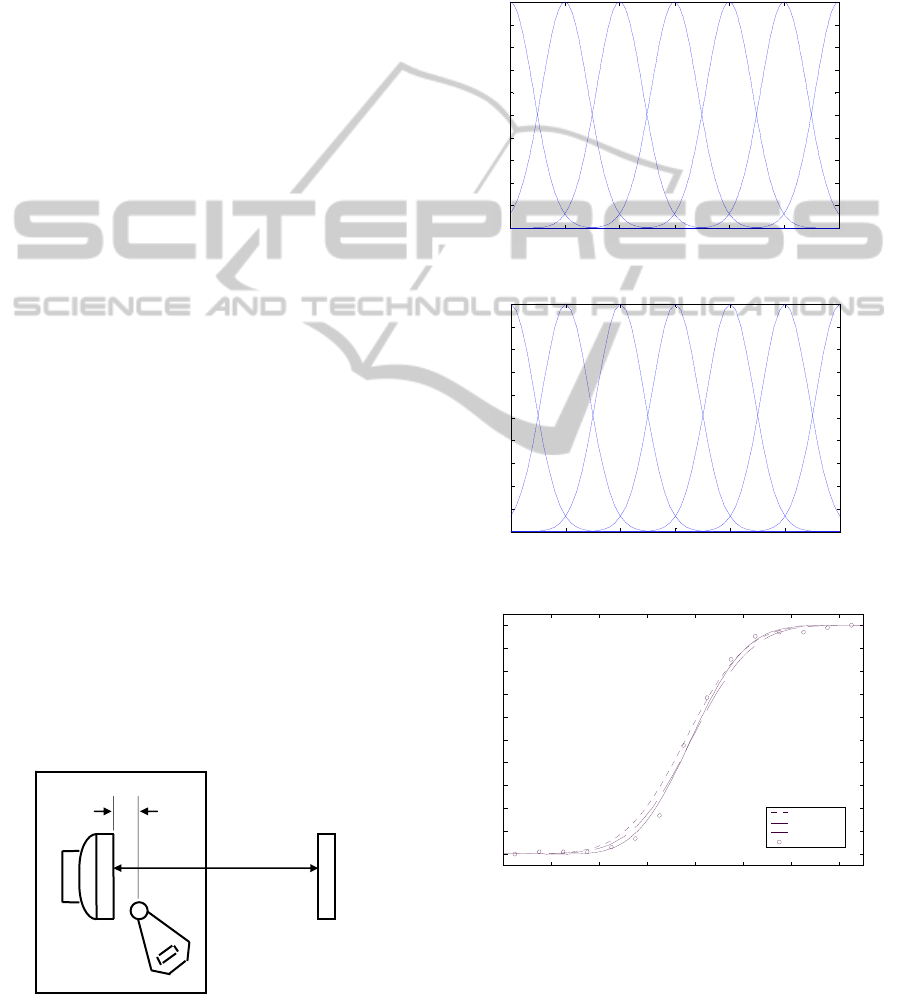
Based on the 400 data points, the expansion
coefficients
mn
A were first estimated by use of (11).
Furthermore, the parameters of the membership
functions in (8) for sound level and electric field
strength with rough quantized levels were decided so
as to express the distribution of data as precisely as
possible, as shown in Figs. 2 and 3. Next, the 200
sampled data within the different time interval which
were non-stationary different from data used for the
estimation of the expansion coefficients were
adopted for predicting the probability distributions
of (i) the electric field based on sound and (ii) the
sound based on electric field.
Figure 1: A schematic drawing of the experiment.
The experimental results for the prediction of
electric field strength and sound level are shown in
Figs. 4 and 5 respectively in a form of cumulative
distribution. From these figures, it can be found that
the theoretically predicted curves show good
agreement with experimental sample points by
considering the expansion coefficients with several
higher orders.
55 60 65 70 75 80 85
0
0.1
0.2
0.3
0.4
0.5
0.6
0.7
0.8
0.9
1
Sound Level [dB]
Figure 2: Membership function of sound level.
2.3 2.4 2.5 2.6 2.7 2.8 2.9
0
0.1
0.2
0.3
0.4
0.5
0.6
0.7
0.8
0.9
1
Electric Field Strength [v/m]
Figure 3: Membership function of electric field.
2.4 2.5 2.6 2.7 2.8 2.9 3 3.1
0
0.1
0.2
0.3
0.4
0.5
0.6
0.7
0.8
0.9
1
Electric Field Strength [v/m]
Cumulative Distribution
1stApprox.
2ndApprox.
3rdApprox.
True values
Figure 4: Prediction of the cumulative distribution for the
electric field strength based on the fuzzy observation of
sound.
For comparison, the generalized regression
analysis method (Ikuta et al., 1997) without using
Electromagnetic
Field Survey
Meter
500mm
Sound Leve
l
Meter
Personal
Computer
20mm
FCTA2014-InternationalConferenceonFuzzyComputationTheoryandApplications
10
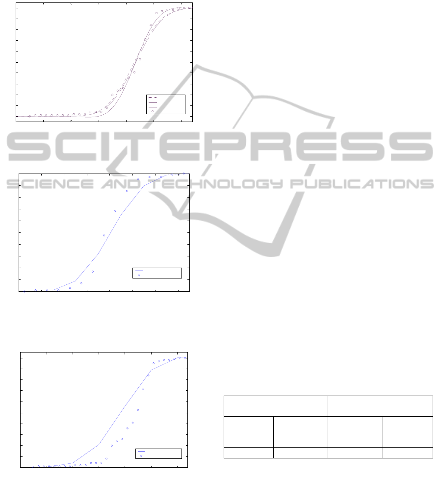
fuzzy theory was applied to the fuzzy data
X
and
Y
. The prediction results are shown in Figs. 6 and 7.
As compared with Figs. 4 and 5, it is obvious that
the proposed method considering fuzzy theory is
more effective than the previous method.
55 60 65 70 75 80 85
0
0.1
0.2
0.3
0.4
0.5
0.6
0.7
0.8
0.9
1
Sound Level [dB]
Cumulative Distribution
1stApprox.
2ndApprox.
3rdApprox.
True values
Figure 5: Prediction of the cumulative distribution for the
sound level based on the fuzzy observation of electric field.
Figure 6: Prediction of the cumulative distribution for the
electric field strength by use of the extended regression
analysis method.
Figure 7: Prediction of the cumulative distribution for the
sound level by use of the extended regression analysis
method.
4.2 Estimation of Specific Signal in
Sound Environment
In order to examine the practical usefulness of the
proposed dynamic signal processing based on the
fuzzy observation, the proposed method was applied
to the real sound environmental data. The road
traffic noise was adopted as an example of a specific
signal with a complex fluctuation form. Applying
the proposed estimation method to actually observed
data contaminated by background noise and
quantized with 1 dB width, the fluctuation wave
form of the specific signal was estimated. The
statistics of the specific signal and the background
noise used in the experiment are shown in Table 1.
Figures 8-10 show the estimation results of the
fluctuation wave form of the specific signal. In this
estimation, the finite number of expansion
coefficients
)2,(
nmB
mn
was used for the
simplification of the estimation algorithm. In these
figures, the horizontal axis shows the discrete time
k , of the estimation process, and the vertical axis
expresses the sound level taking a logarithmic
transformation of power-scaled variables, because
the real sound environment usually is evaluated on
dB scale connected with human effects. For
comparison, the estimation results calculated using
the usual method without considering any
membership function are also shown in these figures.
Since Kalman’s filtering theory is widely used in the
field of stochastic system (Kalman, 1960; Kalman
and Buch, 1961; Kushner, 1967), this method was
also applied to the fuzzy observation data as a trail.
The results estimated by the proposed method
considering the membership function show good
agreement with the true values. On the other hand,
there are great discrepancies between the estimates
Table 1: Statistics of the specific signal and the
background noise.
Statistics of Specific
Signal
Statistics of Background
Noise
Mean
(watt/m
2
)
Standard
Deviation
(watt/m
2
)
Mean
(watt/m
2
)
Standard
Deviation
(watt/m
2
)
2.9
10
-5
2.8
10
-5
2.9 10
-5
1.4 10
-6
based on the standard type dynamical estimation
method (i.e., Kalman filter) without consideration of
the membership function and the true values,
particularly in the estimation of the lower level
values of the fluctuation.
2.4 2.5 2.6 2.7 2.8 2.9 3 3.1
0
0.1
0.2
0.3
0.4
0.5
0.6
0.7
0.8
0.9
1
Electric Field Strength [v/m]
Cumulative Distribution
Theoretical curve
True values
55 60 65 70 75 80 85
0
0.1
0.2
0.3
0.4
0.5
0.6
0.7
0.8
0.9
1
Sound Level [dB]
Cumulative Distribution
Theoretical furve
True values
FuzzySignalProcessingofSoundandElectromagneticEnvironmentbyIntroducingProbabilityMeasureofFuzzyEvents
11
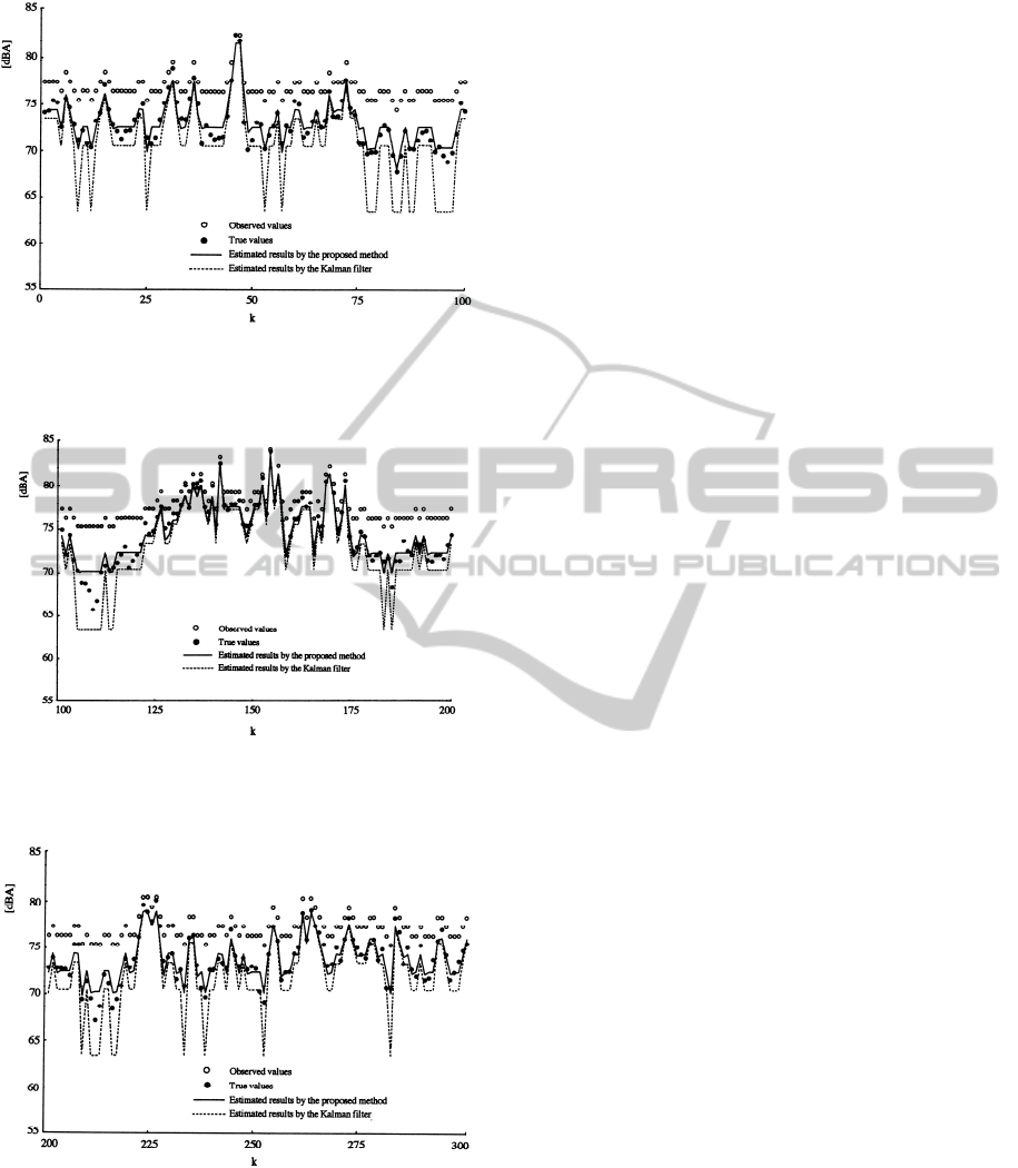
Figure 8: State estimation results for the road traffic noise
during a discrete time interval of [1, 100] sec., based on
the quantized data with 1 dB width.
Figure 9: State estimation results for the road traffic noise
during a discrete time interval of [101, 200] sec., based on
the quantized data with 1 dB width.
Figure 10: State estimation results for the road traffic
noise during a discrete time interval of [201, 300] sec.,
based on the quantized data with 1 dB width.
5 CONCLUSIONS
In this study, new methods for estimating a specific
signal embedded in fuzzy observations have been
proposed within static and dynamic frameworks.
The proposed estimation methods have been realized
by introducing a fuzzy logic approach into the
probabilistic description of the signal. The
effectiveness of the proposed fuzzy signal
processing method has been confirmed
experimentally by applying it to the real sound and
electromagnetic data.
REFERENCES
Bell, B. M., Cathey, F. W., 1993. The iterated Kalman
filter update as a Gaussian-Newton methods. In IEEE
Transactions on Automatic Control, Vol. 38, No. 2, pp.
294-297.
Eykhoff, P., 1984. System identification: parameter and
state estimation, John Wiley & Sons. New York.
Guoshen, Y., 2012. Solving inverse problems with
piecewise linear estimators: from gaussian mixture
models to structured sparsity. In IEEE Transactions on
Image Processing, Vol. 21, No. 5, pp. 2481-2499.
Ikuta, A., Ohta, M., Ogawa, H., 1997. Various regression
characteristics with higher order among light, sound
and electromagnetic waves leaked from VDT. In
Journal of International Measurement Confederation,
Vol. 21, No. 1-2, pp. 25-33.
Ikuta, A., Tokhi, M. O., Ohta, M., 2001. A cancellation
method of background noise for a sound environment
system with unknown structure.In IEICE Transactions
on Fundamentals of Electronics, Communications and
Computer Sciences, Vol. E84-A, No. 2, pp. 457-466.
Ikuta, A., Ohta, M., Siddique, M. N. H., 2005. Prediction
of Probability Distribution for the Psychological
Evaluation of Noise in the Environment Based on
Fuzzy Theory. In International Journal of Acoustics
and Vibration, Vol. 10, No. 3, pp. 107-114.
Julier, S. J., 2002. The scaled unscented transformation. In
Proceedings of American Control Conference, Vol. 6,
pp. 4555-4559.
Kalman, R. E., 1960. A new approach to linear filtering
and prediction problems. In Transactions of the ASME
Series D, Journal of Basic Engineering, Vol. 82, No.1,
pp. 35-45.
Kalman, R. E., Buch, R. S., 1961. New results in linear
filtering and prediction theory. In Transactions of the
ASME Series D, Journal of Basic Engineering, Vol. 83,
No. 1, pp. 95-108.
Kitagawa, G., 1996. Monte carlo filter and smoother for
non-Gaussian nonlinear state space models. In Journal
of Computational and Graphical Statistics, Vol. 5, No.
1, pp. 1-25.
Kushner, H. J., 1967. Approximations to optimal nonlinear
filter. In IEEE Transactions on Automatic Control,
Vol. 12, No. 5, pp. 546-556.
Ohta, M., Koizumi, T., 1968. General statistical treatment
of response of a non-linear rectifying device to a
FCTA2014-InternationalConferenceonFuzzyComputationTheoryandApplications
12

stationary random input. In IEEE Transactions on
Information Theory, Vol. 14, No. 4, pp. 595-598.
Ohta, M., Yamada, H., 1984. New methodological trials of
dynamical state estimation for the noise and vibration
environmental system. In Acustica, Vol. 55, No. 4, pp.
199-212.
Orimoto, H., Ikuta, A., 2014. State estimation method of
sound environment system with multiplicative and
additive noise. In International Journal of Circuits,
Syatems and Signal Processing, Vol. 8, pp. 307-312.
Zadeh, L. A., 1968. Probability measures of fuzzy events.
In Journal of Mathematical Analysis and Applications,
Vol. 23, pp.421-427.
FuzzySignalProcessingofSoundandElectromagneticEnvironmentbyIntroducingProbabilityMeasureofFuzzyEvents
13
