2-D Load Transfer Control Considering Obstacle Avoidance

and Vibration Suppression

Junichi Nakajima and Yoshiyuki Noda

Department of Mechanical Systems Engineering, University of Yamanashi,4-3-11, Takeda, Kofu, Yamanashi, Japan

Keywords:

Load Transfer Control, Trajectory Optimization, Vibration Suppression, Obstacle Avoidance, Overhead

Traveling Crane.

Abstract:

This paper is concerned with an advanced transfer control for load transfer machines such as a crane. In the

load transfer machine, it is required to carry the load efﬁciently and safety. In order to satisfy this requirement,

fast transfer of load, obstacle avoidance and vibration suppression have to be accomplished in the load transfer

system. Therefore in this study, the load transfer control system which the transfer trajectory on a plane is

optimized in consideration of the vibration suppression, obstacles avoidance and fast transfer is proposed.

Moreover, in order to optimize the trajectory in a short time, the fast solution approach is also proposed in

this study. The effectiveness of the proposed transfer control system is veriﬁed by the experiments using the

laboratory type overhead traveling crane system.

1 INTRODUCTION

In manufacturing and construction industries, a load

transfer machine such as an overhead traveling crane

and a gantry loader is used to carry a heavy load and

to support the assembly of components. These trans-

fer machines are required to reach at the target po-

sition in a short time and to avoid the obstacles on a

plane(Kawakami, et al., 2003), (Negishi, et al., 2013).

Furthermore, it is required to suppress the vibration of

the transfer object in the overhead traveling crane and

the gantry loader, because the next task after arriving

at the target position is delayed by the vibration oc-

curred. Therefore, there is a great hope that the load

transfer machine has the control functions of the ob-

stacles avoidance, the vibration suppression and fast

transfer(Yano, et al., 2002).

In order to fulﬁll the above requirements, the

transfer control systems have been proposed in the

previous studies. Especially, a lot of transfer con-

trol systems for an overhead traveling crane have been

proposed. The vibration suppression control to the

load of the overhead crane using optimal control the-

ory was proposed(Al-Garni, et al., 1995). The gain-

scheduled control was applied for suppressing the vi-

bration of the load with rope length varying(Takagi

and Nishimura, 1998), (Harald and Dominik, 2009).

The acceleration of the cart was shaped for elimi-

nating the natural frequency element of the vibra-

tion(Murakami and Ikeda, 2006). However, these

control systems are only for the swaying suppression

of the load. In the 2-D load transfer system such as the

overhead traveling crane without the vertical transfer,

a path planning with obstacles avoidance is needed.

In studies of the path planning for transfer system,

the path of the transfer object was derived by the po-

tential method(Branner,et al., 2012), the probabilistic

road map method(Yu-Cheng, et al., 2012), and pre-

dicting the action of the moving obstacle(Tamura, et

al., 2013). In the study(Suzuki and Terashima, 2000),

the potential method is used for deriving the path with

obstacle avoidance, and the path is reshaped for sup-

pressing the vibration. Since the reshaped path differs

from the path for avoidance of obstacle derived from

the potential method, the transfer object is in danger

of collision with obstacle.

Therefore in this study, the 2-D load transfer con-

trol using the trajectory planning approach consider-

ing the obstacles avoidance, the vibration suppression

and the fast transfer is proposed for the load transfer

machine on a plane. In this approach, the trajectory of

the cart can be derived by the optimization problem

which minimizes the integral square error of the cart

position and the target position, and energy of desired

frequency bands. The natural frequencies of the vi-

bration are assigned to the frequency bands in the cost

function for vibration suppression. The optimization

problem has the constraints on the acceleration, the

653

Nakajima J. and Noda Y..

2-D Load Transfer Control Considering Obstacle Avoidance and Vibration Suppression.

DOI: 10.5220/0005030806530660

In Proceedings of the 11th International Conference on Informatics in Control, Automation and Robotics (ICINCO-2014), pages 653-660

ISBN: 978-989-758-040-6

 2014 SCITEPRESS (Science and Technology Publications, Lda.)

velocity, and the position of the cart. The obstacles

are given as the constraints of the cart position. More-

over, in order to derive the trajectory in a short time,

the fast solution of the trajectory planning is also pro-

posed in this study. The effectiveness of the proposed

transfer control system is veriﬁed by the experiments

using the laboratory overhead traveling crane system.

2 REPRESENTATION OF LOAD

TRANSFER SYSTEM

The load transfer system in this study consists of two

position feedback control systems to the 2-D transfer

machine with an input and state constraints as shown

in Figure 1. These position feedback control systems

are assigned orthogonally in the 2-D load transfer ma-

chine. P(s) is shown as the transfer machine with vi-

bration elements, K(s) is shown as the feedback con-

troller, and r, z

and z

are shown as the target po-

sition, the control input and the controlled variables,

respectively. The observed variable y is the cart po-

sition which measured by the sensor such as a rotary

encorder.

Figure 1: Position feedback control system in load transfer

system

The model to transfer on X-axis in the orthogonal

arrangement is described by the discrete time system

(k + 1) = A

clx

(k) + B

clx

(k), (1)

(k) = C

zclx

(k) + D

zxlx

(k), (2)

(k) = C

yclx

(k) + D

yclx

(k). (3)

Similarly, that on Y -axis is described as

(k + 1) = A

cly

(k) + B

cly

(k), (4)

(k) = C

zcly

(k) + D

zxly

(k), (5)

(k) = C

ycly

(k) + D

ycly

(k). (6)

where x

(k) ⊂ R

and x y(k) ⊂ R

are shown as

the state vectors of each feedback system, and z

(k)

and z

(k) are shown as the control variables with the

constraints on each axis. The equation (1) is the

state equation to transfer on X -axis. The equation (2)

is output equation about controlled variable, and the

equation (3) is the observation equation. The transfer

on Y -axis is described similarly. The initial condition

is as x(0) = 0 becouse of the transfer from a stationary

state, and z

(k) and z

(k) has to be ﬁlled restrictions

(k) ∈ Z

= {z || z

|≤ z

},∀k, (7)

(k) ∈ Z

= {z || z

|≤ z

},∀k, (8)

where z

and z

are the boundary parameters of the

constraints.

3 TRAJECTORY PLANNING

APPROACH

We propose the trajectory planning method with the

time-series information by the optimization problem

which is considered reaching a target position in a

short time, suppressing the vibration, ﬁlling the con-

straints of the transfer machine, and obstacles avoid-

ance for the load transfer system.

3.1 Cost Function

One of the purpose in this study is to minimize the

cost function with the integral square error of the cart

position y and the target position r

in order to trans-

fer the target position in a short time, and the en-

ergy of the frequency bands to the varying natural fre-

quency of the vibration in order to suppress the vibra-

tion which the naturel frequency is changed. The cost

function is shown as

J=w

N−1

∑

k=0

| r

(k) − y

(k) |

N−1

∑

k=0

| r

(k) − y

(k) |

∫

| z

(v) |

dv + w

∫

| z

(v) |

dv. (9)

In this cost function, r

and r

are the target position

on X- and Y -axes, respectively. The ﬁrst term in right

side has the integral square error of the cart position

y and the target position r

, additionally the second

term and the third term are the integral energy of the

frequency bands (v

to v

) on the control input on X-

and Y -axes, respectively. And, w

≥ 0, w

≥ 0 and

≥ 0 are the weight coefﬁcients of scalar. Here,

the control input and the controlled and observation

ICINCO2014-11thInternationalConferenceonInformaticsinControl,AutomationandRobotics

654

valuables can be derived from the equations (2) and

(3) as

(k) =

k−1

∑

i=0

zclx

k−i−1

clx

(i) +D

zclx

(k), (10)

(k) =

k−1

∑

i=0

yclx

k−i−1

clx

(i) + D

yclx

(k). (11)

Here, the vectors of the input and the controlled vari-

able are deﬁned respectively as

= [z

(0) z

(1) · ·· z

(n − 1)]

= [z

(0) z

(1) · ·· z

(n − 1)]

. (12)

Moreover, R

and Y

are the vectors consists of

the elements r

(k)Cr

(k) and y

(k), (k =0,1,·· ·,n-1).

Therefore, the equations (10) and (11) can be repre-

sented as

= M

, Y

= M

, (13)

where M

and M

are shown as







zclx

0 · · · 0

zclx

clx

zclx

· · ·

yclx

n−2

clx

· · · C

zclx

clx

zclx









D 0 · · · 0



(14)

∆ ∆

∆

∆ ∆

∆

∆ ∆

∆

∆ ∆

∆

∆ ∆

∆

∆ ∆

∆

are constant.

Therefore, they are omitted from the cost function.

and these transposes are same

∆ ∆

∆

∆ ∆

∆

∆ ∆

∆

∆ ∆

∆

∆ ∆

∆

∆ ∆

∆

(14)





· · ·











yclx

0 · · · 0

yclx

clx

yclx

· · ·

yclx

n−2

clx

· · · C

yclx

clx

yclx







∆ ∆

∆

∆ ∆

∆

∆ ∆

∆

∆ ∆

∆

∆ ∆

∆

∆ ∆

∆

are constant.

Therefore, they are omitted from the cost function.

and these transposes are same

∆ ∆

∆

∆ ∆

∆

∆ ∆

∆

∆ ∆

∆

∆ ∆

∆

∆ ∆

∆

(15)

Moreover, M

and M

on Y -axis can be derived

by similar process to the derivation on X-axis. There-

fore, the ﬁrst term without the weight coefﬁcient of

the cost function as shown in the equation (9) can be

represented as

= R

− R

+ R

− R

−R

+ R

. (16)

In the equation (16), R

and R

are constant.

Therefore, they are omitted from the cost function.

And, R

(i = x,y) and these transposes are same

value because of scalar. Therefore, the equation (16)

can be organized as

= (R

− 2R

)

+(R

− 2R

). (17)

The second term in right side without the weight co-

efﬁcient w

in the cost function as shown in the equa-

tion (9) can be represented by using discrete Fourier

transform as

∫

| z

(v) |

dv =

∫

N−1

∑

(k)e

− jv∆T k

∫

N−1

∑

k=0

(k)e

− jv∆T k

∗

N−1

∑

k=0

jv∆T k

(k)dv, (18)

where ∆T is a sampling period. By using the equation

(12), the cost function J

can be represented as

∫

∗

dv, (19)

where E is as

E = [1 e

− jv∆T

···e

− jv∆T (n−1)

]

. (20)

∗

is the conjugate transpose matrix of E. Then, the

equation (19) can be represented as

= Z

∫

∗

dvZ

= Z

, (21)

where M

is as

∫

∗

(14)

(15)

-axis can be derived by

-axis. There-

, the ﬁrst term without the weight coefﬁcient of

the cost function as shown in the equation (9) can be







− v

∆T

−e

∆T

j∆T

−

∆T

−e

∆T

j∆T

− v

−

∆T (n−1)

−e

2 jv

∆T (n−1)

j∆T

· · ·

∆T (n−1)

−e

2 jv

∆T (n−1)

j∆T

∆T

−e

∆T

j∆T

−

∆T

−e

∆T

j∆T

− v







. (22)

in the equation (21) can be replaced to the sym-

(22)

in the equation (21) can be replaced to the

symmetric matrix M

shown as

= Z

(

+ M

= Z

(23)

where M

is shown as

are constant.

Therefore, they are omitted from the cost function.

and these transposes are same

value because of scalar. Therefore, the equation (16)

(17)

The second term in right side without the weight co-

in the cost function as shown in the equa-

tion (9) can be represented by using discrete Fourier







− v

sinv

∆T −sin v

∆T

sinv

∆T −sin v

∆T

− v

sinv

∆T (n−1)−sin v

∆T (n−1)

· · ·

sinv

∆T (n−1)−sin v

∆T (n−1)

sinv

∆T −sin v

∆T

sinv

∆T −sin v

∆T

− v







. (24)

(24)

2-DLoadTransferControlConsideringObstacleAvoidanceandVibrationSuppression

655

can be represented as Z

= M

zux

from the

equation (13). Therefore, the second term J

in the

cost function as shown in the equation (9) can be rep-

resented as

= R

zux

. (25)

Going through the same procedure as J

, the third

term J

in the equation (9), which is the integral en-

ergy on the frequency bands (v

to v

) in Y -axis, can

be derived as

= R

zuy

. (26)

Summarizing the equations (17), (25) and (26), the

cost function in the equation (9) can be represented as

min

J=min

+ w

)

=min

{−2w

+ R

)

+ w

zux

+ w

zuy

}. (27)

This cost function has the dynamics of the transfer

system as represented in equation (13).

3.2 Input and State Constraints on

Transfer System

From the equations (7) and (8), the input and state

constraints of the 2-D load transfer machine can be

represented as

| M

zxx

|≤ Z

xxc

,| M

zux

|≤ Z

uxc

, (28)

| M

zxy

|≤ Z

xyc

,| M

zuy

|≤ Z

uyc

, (29)

where Z

xxc

, Z

xyc

, Z

uxc

and Z

uyc

are the input and state

constraints as

xxc

= [z

··· z

]

, Z

xyc

= [z

··· z

]

xuc

= [z

uxc

··· z

uxc

]

, Z

uyc

= [z

uyc

··· z

uyc

]

. (30)

The trajectory planning in this study is performed on

the ﬁnite time interval. In order to reach the transfer

object to the target position (r

, r

) with stationary

at the ﬁnal time, the following equality constraints are

given.

f x

= Z

f x

, M

f y

= Z

f y

, (31)

where M

f x

, M

f y

, Z

f x

and Z

f y

are as

f x



yclx

N−2

clx

···C

yclx

clx

yclx

zclx

N−2

clx

···C

zclx

clx

zclx



, (32)

f y



ycly

N−2

cly

···C

ycly

cly

ycly

zcly

N−2

cly

···C

zcly

cly

zcly



, (33)

f x





, (34)

f y





. (35)

The ﬁrst, second and third rows in the equation (31)

are for the terminate constraints of the cart position,

velocity and acceleration, respectively. The reference

trajectory optimization using the equations (27), (28),

(29) and (31) is performed by a quadratic program-

ming. However, since the reference trajectories on

X- and Y -axes are designed independently, it does not

include the function of the obstacle avoidance. In

next section, we introduce the function of the obstacle

avoidance.

3.3 Obstacle Represented by Constraint

Condition

If we try to apply for the load transfer system such

as an overhead traveling crane with some obstacles

in the transfer space, we should design 2-D transfer

trajectory which avoids the obstacles and does not ex-

cite the vibration. Therefore in this study, the obsta-

cle area are deﬁned as inequality constraints in the

quadratic form, and they are given into the optimiza-

tion problem shown in the previous section for plan-

ning the trajectory with the obstacles avoidance.

Figure 2: Path planning with obstacle avoidance.

In this approach, the obstacle is covered in the

ellipse as shown in Figure 2. The inside of the el-

lipse is the no penetration area for planning the trajec-

tory. Therefore, the following inequality constraint is

given.

(k) − x

)

(k) − y

)

− 1 ≥ 0, (36)

where (x

) is shown as the center position of the

ellipse, and a and b are shown as the length of the X-

and Y -directions on the ellipse. For matrix represen-

tation of the equation (36), the following inequality

equation is deﬁned.

ICINCO2014-11thInternationalConferenceonInformaticsinControl,AutomationandRobotics

656

− e

)

− e

)/(a

)

+(e

− e

)

− e

)/(b

) − 1

= (R

− 2X

)/(a

) + (R

−2Y

)/(b

) − 1 ≥ 0, (37)

where e

= [1,0, 0,0, ··· , 0] ∈ R

1×n

, X

,· ·· ,x

]

∈ R

1×n

, Y

= [y

,· ·· ,y

]

∈ R

1×n

The equation (37) shows the inequality equation at

k = 1. At k = 2, e

= [0,1,0, 0,· ·· ,0] ∈ R

1×n

is applied as the equation (37). Therefore,

= [0,·· · ,0,1, 0,· ·· ,0] ∈ R

1×n

is deﬁned for

applying all of trajectory. The inequality constraint

for obstacle avoidance is represented as

ηM

− 2X

ηM

ηX

)/(a

) + (R

ηM

−2Y

ηM

ηY

)/(b

) −

η ≥ 0, (38)

where,

η = [e

···e

]

, (39)

η = [e

···e

]

. (40)

Organizing the equation (38) into a quadratic form,

the following equation can be derived.

(

ηM

+ R

(

ηM

−(

ηM

− (

ηM

≥ −

ηX

−

ηY

η (41)

By adding the equation (41) into the trajectory opti-

mization in the previous section, the 2-D trajectory

with function of the obstacles avoidance can be de-

rived.

Therefore, the trajectory planning problem of the

2-D load transfer machine that is concerned with fast

transfer control with vibration suppression and ob-

stacles avoidance to a transfer object is resulted a

quadratic programing problem with quadratic con-

straints. This quadratic programming problem can

be solved by a sequential quadratic programming

method.

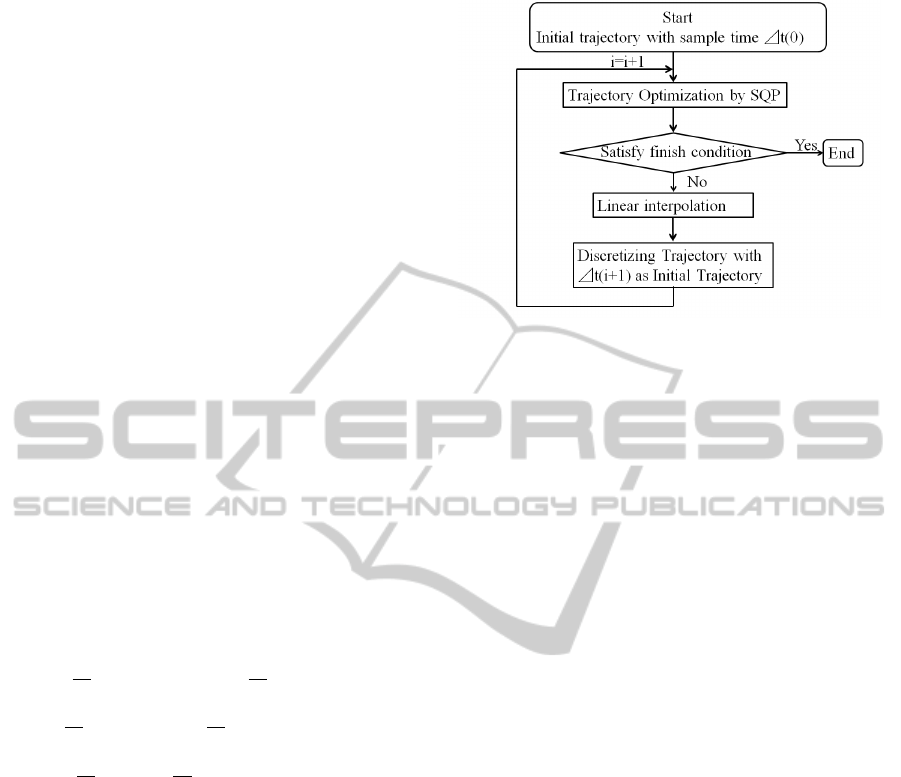
4 FAST SOLUTION OF

TRAJECTORY PLANNING

In this trajectory planning method proposed in this

study, the calculation takes immense amount of time,

Figure 3: Iteration for fast solution of transfer trajectory.

because the trajectory represented by the sample num-

ber n should be solved by the quadratic programming

problem with the quadratic constraints. In order to

solve the problem in a short time, we propose the fast

solution of the trajectory planning.

The calculation time for planning the trajectory

is decreased with decreasing the sample number n.

Therefore, the fast solution method as shown in Fig-

ure 3 is proposed. In this method, the trajectory with

the long sampling period is derived by the trajectory

planning proposed in the previous section. Then, the

discrete trajectory with the long sampling period is

linearly-interpolated, and the interpolated trajectory is

discretized with the shorter sampling period than that

of the previous optimized trajectory. The trajectory

optimization is performed with the discretized trajec-

tory as the initial trajectory. By iterating the proce-

dure as shown in Figure 3, the trajectory with a lot

of sample number n can be optimized in a short time.

The terminal condition in the iteration is given as

| J

(i − k) − J

(i − k − 1) |< ξ, k = (0, 1,2), (42)

where,

= J/n. (43)

J is the cost function as shown in the equation (27).

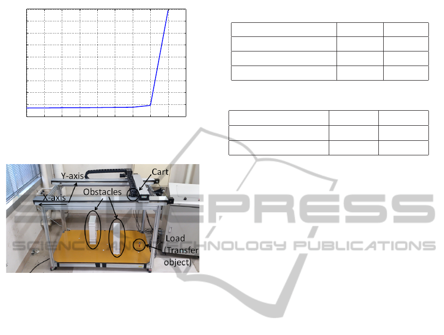
n is the sample number. Here, the relation between

the evaluation value J

and the sampling period ∆t

is shown in Figure 4. As seen from Figure 4, the

evaluation J

is converged with decreasing the sam-

pling period ∆t. Therefore, the trajectory is optimized

quickly by giving the appropriate ﬁnish condition. In

this study, we deﬁne the ﬁnish condition with ξ = 0.1,

that is selected by the relation between the evaluation

and the sampling period ∆t as shown in Figure 4.

2-DLoadTransferControlConsideringObstacleAvoidanceandVibrationSuppression

657

0.1 0.2 0.3 0.4 0.5 0.6 0.7 0.8 0.9 1

−5

Sampling Period[s]

Evaluation Js

Figure 4: Relation between evaluation J

and sampling pe-

riod.

Figure 5: Overhead traveling crane system.

5 EXPERIMENTAL VALIDATION

USING OVERHEAD

TRAVELING CRANE

The effectiveness of the proposed method is validated

by the experiments using laboratory overhead travel-

ing crane as shown in Figure 5. The load as the trans-

fer object is suspended to the cart by the rope. The

travel range of the cart on X- and Y -axes are 1.2[m]

and 0.5[m], respectively. And the maximum rope

length is 0.85[m]. The cart traveled on X- and Y -axes

is driven by a servomotor and a belt-and-pulley mech-

anism on each axis. The rope is reeled by a servomo-

tor and a pulley. The cart position can be detected by

rotary encoders attached to the servomotor on each

axis. The rope length can also be detected by a rotary

encoder attached the servomotor. The sway angle of

the rope with the load can be detected by a laser range

sensor system. The constraints to the cart transfer are

shown in Table 1. The time constants and the gains

of the motors represented as a ﬁrst order delay system

are shown in Table 2. The position feedback control

systems are constructed to the motors on X- and Y -

axes, respectively. The proportional control with the

both gains, K

= 100 are applied to the position feed-

back control systems.

Table 1: Constraints of transfer system.

Table 1: Constraints of transfer system

X-axis Y-axis

Velocity[m/s] ±0.35 ±0.35

Acceleration[m/s

] ±0.5 ±0.5

Input voltage[V] ±10 ±10

5 EXPERIMENTAL VALIDATION

Table 2: Parameters of motors.

Table 2: Parameters of motors

X-axis Y-axis

Gain[m/s/V] 0.0361 0.0358

Time constant[s] 0.011 0.015

The experimental conditions to the laboratory

overhead traveling crane system are shown as follows.

• Target position of the cart transfer is located as

1.0[m] and 0.4[m] on the X- and Y -axes, respec-

tively.

• The range of the rope length while the cart trans-

fer is between 0.3[m] and 0.7[m]. Therefore, the

natural angular frequency of the load vibration is

varied between 3.74[rad/s] and 5.72[rad/s]. The

frequency band for suppressing the vibration is set

to the range between 3.74[rad/s] and 5.72[rad/s]

in the trajectory planning of the cart transfer on

X- and Y -axes.

• Two obstacles covered into the ellipses are put

into the transfer space. The size of the obstacles

are same as 0.08[m] length of ellipse on X -axis

and 0.25[m] length on Y -axis. The center posi-

tions of the ellipses are located on [0.35 0] and

[0.75 0.4].

• The weight coefﬁcients are given as w

= 1, w

1 and w

= 1 in case of the trajectory considering

with the vibration suppression. For comparison,

another experiment with the weight coefﬁeients

= 1, w

= 0 and w

= 0, is performed. It is

not considered with the vibration suppression.

• The transfer time is set to 6[s], and the sampling

period on the transfer control is 0.01[s].

In the procedure of the fast solution as shown in Fig-

ure 3, the series of the sampling period for optimizing

is given as ∆t = [1 0.5 0.25 0.1]. And in the terminal

condition shown in the equation (42), the evaluation

is selected as k = 0.

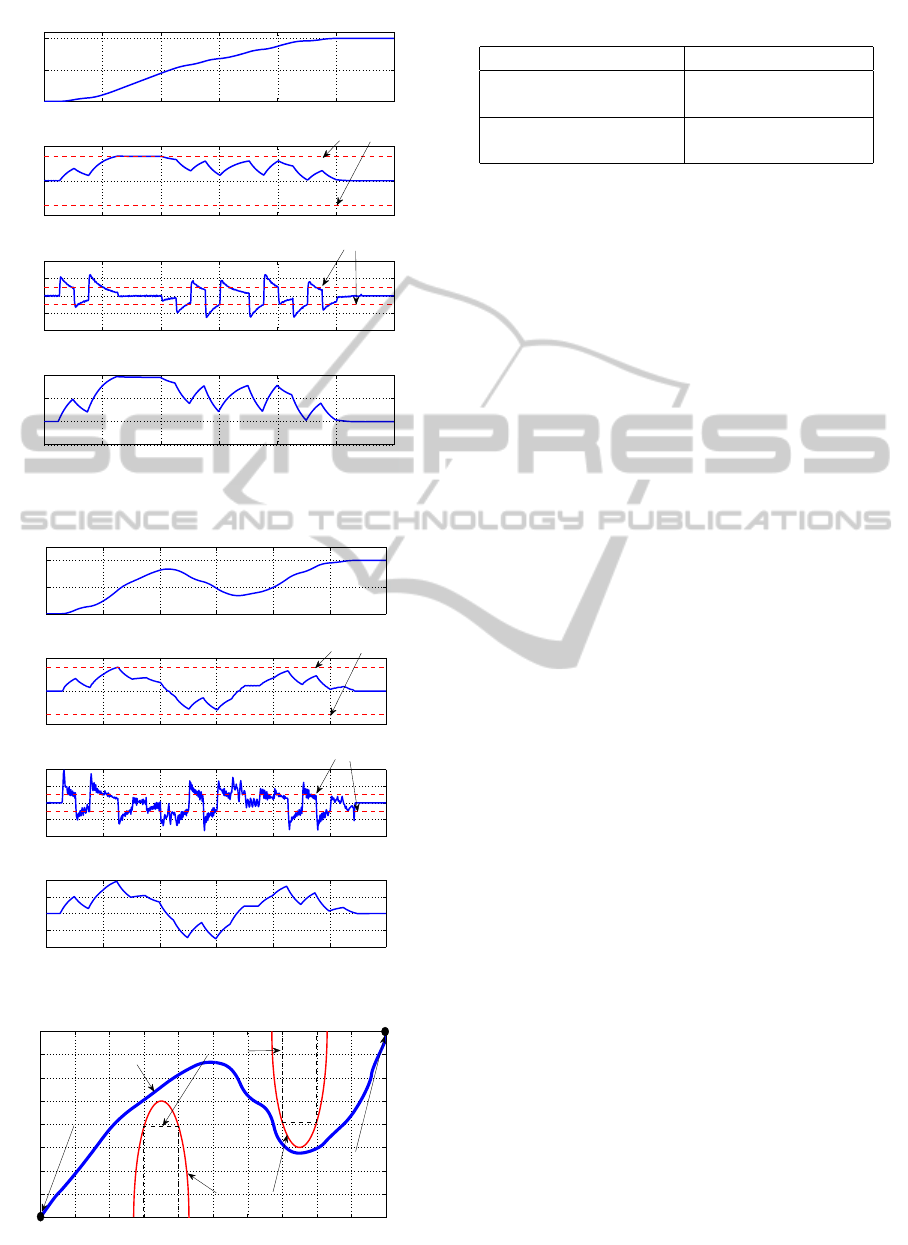
The experimental results of the cart transfer on X -

and Y -axes are shown in Figures 6 and 7, respectively.

In these ﬁgures, (a), (b), (c) and (d) show the cart posi-

tions, the velocities, the accelerations and the control

inputs, respectively. In (b) and (c), the broken lines

ICINCO2014-11thInternationalConferenceonInformaticsinControl,AutomationandRobotics

658

0 1 2 3 4 5 6

0.5

Position[m]

Time[s]

0 1 2 3 4 5 6

−0.5

0.5

Velocity[m/s]

Time[s]

0 1 2 3 4 5 6

−2

−1

Acceleration[m/s

]

Time[s]

0 1 2 3 4 5 6

−5

Control input[V]

Time[s]

Constraints

(a)

(b)

(c)

(d)

Figure 6: Experiment results on X-axis.

0 1 2 3 4 5 6

0.2

0.4

Position[m]

Time[s]

0 1 2 3 4 5 6

−0.5

0.5

Velocity[m/s]

Time[s]

0 1 2 3 4 5 6

−2

−1

Acceleration[m/s

]

Time[s]

0 1 2 3 4 5 6

−10

−5

Control input[V]

Time[s]

Constraints

(a)

(b)

(c)

(d)

Figure 7: Experiment results on Y-axis.

0 0.1 0.2 0.3 0.4 0.5 0.6 0.7 0.8 0.9 1

0.05

0.1

0.15

0.2

0.25

0.3

0.35

0.4

x−position

y−position

Trajectory of cart

Start position

Target position

Obstacles

No penetrations

Figure 8: Experiment results in transfer trajectory.

Table 3: Calculation times.

Computation time[s]

Conventional solution 1484.00

(Once optimization)

Fast solution proposed 5.85

in this study

are the constraints to each state. The control inputs

are within the constraints. However, the velocities

and the accelerations are exceeded. In this approach,

since the sample period in the trajectory derived from

the terminal condition in the fast solution is longer

than that of the transfer control, the sample period of

the trajectory is adjusted to that of the controller by

the linear-interpolation method. By this procedure,

the velocities and the accelerations can be exceeded.

In order to solve this problem, interpolating smoothly

the trajectory will be required in the future.

The trajectory on X- and Y -axes is shown in Fig-

ure 8. In Figre 8, the blue bold line is the trajectory

of the transfer object, and the red thin lines are the

no penetration areas. The black broken lines show

the edges of the obstacles. As seen from Figure 8,

the transfer object avoids the obstacles, and reachs

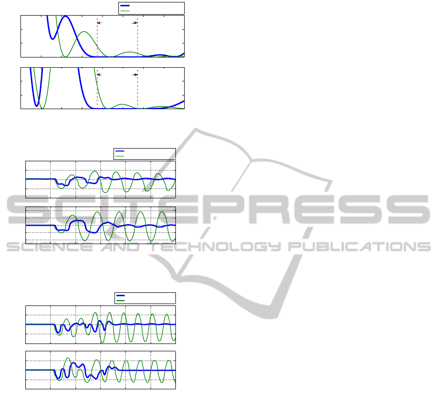
the target position. The power spectrum of the in-

put control is shown in Figure 9. The blue bold lines

show the control input considering the vibration sup-

pression, and the green thin lines show the that with-

out the vibration suppression. In the power spectrum

of the frequency bands 3.74[rad/s] to 5.72[rad/s], the

spectrum with considering the vibration suppression

is reduced. Therefore, the vibration considered in the

proposed method can not be excited. The experimen-

tal results of the vibrations with the natural angular

frequencies 3.74[rad/s] and 5.72[rad/s] are shown in

Figures 10 and 11, respectively. The blue bold lines

show the results by the proposed method considering

vibration suppression, and the green thin lines show

the results without vibration suppression. In Figures

10 and 11, it is seen that the vibration is suppressed

by the proposed method. The calculation time com-

pared between the fast solution proposed in this study

and the conventional solution which the trajectory op-

timization is performed only once by the sample pe-

riod 0.01[s], as shown in Table 3. The proposed opti-

mization process is much faster than the conventional

optimization process.

6 CONCLUSIONS

We proposed the trajectory planning method for 2-

D load transfer machine including vibration element.

2-DLoadTransferControlConsideringObstacleAvoidanceandVibrationSuppression

659

0 1 2 3 4 5 6 7 8

Power spectrum on X− axis

With vibration suppression

Without vibration suppression

0 1 2 3 4 5 6 7 8

Power spectrum on Y− axis

Frequency[rad/s]

Suppression band

Figure 9: Power spectrums of control inputs.

0 2 4 6 8 10 12

−0.4

−0.2

0.2

0.4

Sway angle (X−axis) [rad]

With vibration suppression

Without vibration suppression

0 2 4 6 8 10 12

−0.4

−0.2

0.2

0.4

Time [s]

Sway angle (Y−axis) [rad]

Figure 10: Experiment results of vibration with natural an-

gular frequency 3.74[rad/s] (Rope length:0.7[m]).

0 2 4 6 8 10 12

−0.4

−0.2

0.2

0.4

Sway angle(X−axis) [rad]

With Vibration suppression

Without vibration suppression

0 2 4 6 8 10 12

−0.4

−0.2

0.2

0.4

Sway angle(Y−axis) [rad]

Time [s]

Figure 11: Experiment results of vibration with natural an-

gular frequency 5.72[rad/s] (Rope length:0.3[m]).

The proposed method makes the transfer object avoid

the obstacles, the motion suppress the vibration in the

transfer object, and the state and the control input

keep under the constraints. Moreover, the fast solu-

tion which shorten the calculation time of the trajec-

tory optimization has been proposed in this study. In

the experiments for validating the proposed method, it

was seen that the vibration suppression, the obstacles

avoidance are accomplished. In the future works, we

will discuss the smooth interpolation method so that

the velocity and the acceleration of the transfer object

fall within the constraints.

REFERENCES

Kawakami, S, Miyoshi, T and Terashima, K, Path Planning

of Transferred Load Considering Obstacle Avoidance

for Overhead Crane, System Integration Division An-

nual Conference, p.640-641, 2003

Negishi, M, Masuda, H, Ohsumi, H and Tamura, Y, Eval-

uation of overhead crane trajectory, JSME Confer-

ence on Robotics and Mechatronics, p.1A2-p19(1)-

(4), 2013

Yano, K, Eguchi, K and Terashima, K, Sensor-Less Sway

Control of Rotary Crane Considering the Collision

Avoidance to the Ground, Transactions of the Japan

Society of Mechanical Engineers, Series(C), Vol. 68,

No. 676, p.146-153

A. Z. Al-Garni, K. A. F. Moustafa and S. S. A. K. Javeed

Nizami, Optimal Control of Overhead Cranes, Con-

trol Eng. Practice, Vol.3, No.9, p.1277-1284, 1995

Takagi, K, and Nishimura, H, Gain-Scheduled Control of A

Tower Crane Considering Varying Load-Rope Length,

Transactions of the Japan Society of Mechanical En-

gineers, Series(C), Vol. 64, No. 626, p.113-120

Harald, A and Dominik, S, Passivity-Based Trajectory Con-

trol of and Overhead Crane by Interconnection and

Damping Assignment, Motion and Vibration Control

, p.21-30, 2009

Murakami, S and Ikeda, T, Vibration suppression for High

Speed Position Control of overhead Traveling Crane

by Acceleration Inputs, Dynamics & Design Confer-

ence, p.128(1)-(6), 2006

Brunner, M, Bruggemann, B, and Schulz, D, Autonomously

Traversing Obstacle: Metrics for Path Planning of

Reconﬁgurable Robots on Rough Terrain, Proceed-

ings of 9th International Conference on Informatics in

Control, Automation and Robotics, p.58-69, 2012

Yu-Cheng, C, Wei-Han, H, Shin-Chung, K, A fast path

planning method for single and dual crane erections,

Automation in Construction, Volume 22, p. 468-480,

2012

Tamura, Y, Hamasaki, S, Yamashita, A and Asama, H,

Collision Avoidance of Mobile Robot Based on Pre-

diction of Human Movement According to Environ-

ments, Transactions of the Japan Society of Mechani-

cal Engineers, Series(C), Vol. 79, No. 799, p.617-628

Suzuki, M and Terashima, K, Three Dimensional Path

Planning using Potential Method for Overhead Crane,

Journal of Robotics Society of Japan, Vol.18, No.5,

p.728-736, 2000

ICINCO2014-11thInternationalConferenceonInformaticsinControl,AutomationandRobotics

660