
A Possibility of Fast Running of Tyrannosaurus rex by the Result of
Evolutionary Computation
Yoshiyuki Usami
Institute of Physics, Kanagawa University, Rokkakubash, Yokohama 221-8686, Japan
Keywords: Dinosaur, Locomotion, Evolutionary Computation, Simulated Annealing, Tyrannosaurus.
Abstract: The author examined the effectiveness of the optimization strategy of evolutionary computation and the
conventional simulated annealing method when studying the locomotor motion of bipedal animals. The
simulated annealing method is known as a powerful tool for finding near-optimal solutions for
combinatorial problems such as the NP-complete problem. However, the author found the evolutionary
computational strategy more effective at finding near-optimal solutions of the running motion of bipedal
animals. The author conducted extensive simulations of the running motion of the large, bipedal dinosaur
Tyrannosaurus rex based on realistic, biological parameters. The author’s simulations found that T.rex
could run quickly, up to 14 m/s, which is faster than the beings.
1 INTRODUCTION
Simulated annealing is well known as a powerful
simulation technique for obtaining near-optimal
solutions for combinatorial problems such as the
NP-complete problem, which is typically a traveling
salesman problem (TSP) (Usami and Kano, 1995;
Usami and Kitaoka, 1997). Furthermore, the
statistical physics theory has proven that a slow
annealing schedule leads to a near-optimal solution.
Regarding TSP, the simulated annealing method is
said to be equally appropriate with evolutionary
computation methods such as the genetic algorithm
(GA) (Holland, 1992; Goldberg, 1989). In addition,
it is easier to solve TSP in program coding by using
simulated annealing rather than GA.
On the contrary, the evolutionary computation
strategy is known to be applicable to a variety of
optimization problems. For example, the
evolutionary computation strategy has been used in
searching for a near-optimal solution of animal
locomotion (Sellers and Manning, 2009; Usami et al.,
1998). In this paper, the author has tested the
conventional simulated annealing method and the
evolutionary computation method to obtain the
locomotion pattern of a bipedal animal.
Consequently, the author found that evolutionary
computation is more effective than the simulated
annealing technique in this case. The reason may lie
in the parameter dependence sensitivity of the total
system; a slight change in the parameters induces
large changes in the locomotion pattern.
On the basis of this finding, the author conducted
extensive simulations to determine the running
motion of the bipedal carnivorous dinosaur
Tyrannosaurus rex (T.rex). T.rex is the largest
bipedal theropod that lived in the Cretaceous period
(145–66 million years ago (Ma)). Its maximum
estimated weight was up to 8 tons (Hutchinson et al.,
2011). In 2002, Hutchinson and Garcia published a
paper titled, “Tyrannosaurus was not a fast runner”
(Hutchinson and Garcia, 2002). They assumed
several patterns of midstance posture in running
motion and calculated the required muscle mass to
hold that posture. Using the Froude number (Fr =
v
2
/hg, where v, h, and g represent velocity, hip
height, and the gravity constant, respectively), they
stated that T.rex could not run at a speed of 20 m/s
(Alexander, 1976, 1983, 1989, 2006). However,
their discussion was based on static mechanics; no
explicit speed estimation was involved in the
framework of their study. In 2009, Sellers and
Manning reported the first numerical simulation
study for this problem. They published a result
stating that a running speed of 9–10 m/s was
possible for T.rex. However, a faster running speed
would have been problematic (Fig.1).
In this paper, the author presents the numerical
simulation results of T.rex’s running motion. The
simulation methodology is compared with the
145
Usami Y..
A Possibility of Fast Running of Tyrannosaurus rex by the Result of Evolutionary Computation.
DOI: 10.5220/0005031701450152
In Proceedings of the International Conference on Evolutionary Computation Theory and Applications (ECTA-2014), pages 145-152
ISBN: 978-989-758-052-9
Copyright
c
2014 SCITEPRESS (Science and Technology Publications, Lda.)
simulated annealing and evolutionary computation
methods, and the results of extensive numerical
simulations are presented.
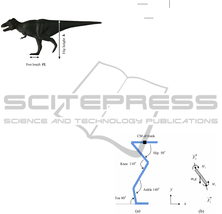
Figure 1: Tyrannosaurus rex and its hip height.
2 SIMULATION OF T. REX’S
RUNNING MOTION
2.1 Mechanics
The motion of running is a periodic one; hence,
expressing the time change of each joint angle using
the Fourier expansion series is appropriate. The
validity of this method was checked in advance
using human locomotion. A human’s running
motion was captured by a combination of optical
measurements and the use of a force plate on the
ground. These data were analyzed by the reliable
system VICON (Vicon Motion Systems). The time
change of each joint angle was expressed using the
Fourier expansion series. Convergence within 1%
accuracy was checked, taking into account the 5th
order of the Fourier expansion. Thus, expressing the
5th order of the Fourier expansion is a good method
for describing the periodic motion of each joint.
For the i-th joint angle, the expansion is expressed
as follows:
)sin()0sin()(
1100
iiiii
tatat
)5sin(
55
ii
ta
,
(1)
where
j
i
a
and
j
i
are the amplitude and the phase of
the j-th order of the expansion series for the i-th
angle, respectively and
is the angular velocity.
The segmented structure of T.rex is the same as that
of Hutchinson and Garcia’s model, shown in Fig. 2
(a).
To study time-dependent dynamics, a solid
object model is used to describe the motion of the T.
rex limb. Namely, the T.rex model moves as one
solid object for the external force according to the
following equations:
)(
2
2
rFgm
dt
Xd
m
y
bodybody
,
(2)
)(
2
2
rFr
dt
Φd
I
,
(3)
where
X
are
Φ
the position vector of the center of
mass and the rotational angle of the object,
respectively. The calculation is achieved in the
sagittal plane, i.e., two-dimensional space x
(horizontal) and y (vertical). I, g, and
)(rF
are T.
rex’s momentum of inertia, the gravitational
constant, and the position vector to the point of the
force, respectively. The second term in Eq. (2)
expresses the fact that gravitational force acts in
vertical direction y. The value of inertia I in this
work is chosen to be I = 19000
2
mkg
. Note that
Hutchinson et al.’s value is I
zz
= 19200
2
mkg
for a
6583 kg T.rex, where I
zz
is the inertia around the axis
perpendicular to the sagittal plane (Hutchinson et al.
2007). The value Bates et al. used is 18890.29
2
mkg
for the “HAT” (Head-Arms-Torso) of a 6071.82 kg
T.rex (Bates et al. 2009).
Figure 2: Segment model of a T.rex leg (a) and a free-body
diagram (b). The angle denoted in (a) represents the best
guess model in the reference (Hutchinson and Garcia,
2002).
Both studies used the same T.rex specimen, MOR
555; however, different reconstructions led to their
slightly different estimations of inertia. The author’s
value is set close to these values. A solid object
model is simple, yet is also known to express the
dynamics of a moving object with many degrees of
freedom (Usami et al., 1998).
To calculate joint torque, or the moment of force
about the joint, a free-body diagram analysis is
applied, as shown in Fig. 2 (b). For example, call the
foot segment “segment 1”, and define the mass and
ECTA2014-InternationalConferenceonEvolutionaryComputationTheoryandApplications
146

moment of inertia as m
1
and I
1
, respectively. The
equations of motion for translation and rotation then
become as follows in the (x, y) plane:
11121
amgmFF
y
,
(4)
11212211
IMMFxFx
gg
,
(5)
where
1
F
,
2
F
, and
1
a
are the force from the
downside segment, the force from the upper
segment, and acceleration, respectively. For
rotational motion,
g
x
1
and
g
x
2
are the vectors from
the center of mass of the 1-th segment to the points
of acting force
1
F
and
2
F
. M
1
and M
2
are the
moments of force between the 0-th and 1-th and the
1-th and 2nd segments, respectively. For the case of
the 1-st segment,
1
F
corresponds to the ground
reaction force and
1
is the time derivative of the
angular velocity. Inserting known terms
1
F
,
1
a
,
1
,
and M
1
into Eq. (5) yields unknown terms
2
F
and
M
2
. Thus, we obtain the moment of force on the
upper segment.
Solid object approximation is used to find the
motion of the whole body. In the expression, the
total mass M, moment of inertia I, and gravitational
constant g are 6071 kg, 9.80 m/s
2
, and 19000
2
mkg
,
respectively. The external force is the ground
reaction force (GRF), which acts in vertical direction
y according to the relation
yy
vkyyF
)(
, where
y and v
y
are the depth from the horizontal level and
the vertical velocity, respectively. This relation is
composed using Hooke’s law with spring constant k
= 1.0 × 10
7
N/m, dumping term with coefficient γ =
2.0 × 10
5
Ns/m in our simulation. This model gives
an appropriate solution of running motion with a
wide range of parameters k and γ in the simulation.
2.2 Evolutionary Computation Method
The next task is searching the optimal Fourier
coefficient for running motion; other parameters are
fixed in the simulation. Using the computational
method to obtain the optimal solution when there are
many degrees of freedom is usually not an easy task;
therefore, a variety of approximation methods have
been proposed in many research areas. One of the
most famous and well-studied methods is the genetic
algorithm (GA) (Fraser and Burnell, 1970; Holland,
1975; Goldberg, 1989). Numerous studies have been
published in many research areas concerning GA,
which is based on the idea of gene evolution, as
observed in actual life systems. In this method, a
digitized virtual gene is introduced and its evolution
is simulated. The virtual gene falls into a stable state
in which the value of evaluation function has a local
minimum. However, the introduction of virtual
genes is unnecessary for this study. Therefore,
looking for another convenient approximation
method is appropriate.
Another approximation method for obtaining a
near-optimal solution is the evolutionary
computation method (Sellers and Manning, 2009;
Usami, 1998; Fogel, 1995). This method is as well
known as the genetic algorithm method when
searching for near-optimal solutions. The
evolutionary computation method does not introduce
a digitized virtual gene but changes system
parameters directly. Parameters rapidly converge
into the local minimum and the result is usually
satisfactory. The evolutionary computation method
is used on this problem.
First, several typical patterns of the running
motion were created using the 3D software 3ds Max
(from Autodesk). The typical patterns include
various motions from flexed to upright. Next, we
apply the dynamical simulation described above. At
the first stage of evolutionary computation, the T.
rex model usually falls on the ground in the
simulation space. The parameters are then improved
by the evolutionary computation method. The
original set of parameters is slightly and randomly
changed within a certain range.
These sets of
parameters are referred to as the children of the
original parent set. Running motions with slightly
changed parameters are calculated, and the best
performing child is selected. The parent of the best
performing parameter set again has children who
have slightly different values from the parent; thus,
the near-optimal solution for running motion is
obtained as a result of the evolutionary computation
method.
The simulation has many choices for the
evaluation function to choose from when obtaining
the appropriate solution and many function types
were tried. Consequently, choosing between running
motion as the product of ground reaction force or of
forward velocity is suitable for this problem’s
evaluation function. This is mainly due to the fact
that the legs of the segment model inevitably rotate
around each joint, thus generating a driving force to
move in any direction. Taking this condition then
yields a smooth running motion for the segment
model of T. rex.
A result of simulated annealing method is
compared to the one of evolutionary computation
method, which is shown in Fig.3. The simulation is
APossibilityofFastRunningofTyrannosaurusrexbytheResultofEvolutionaryComputation
147
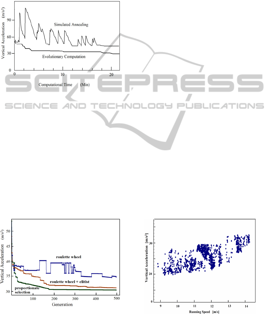
meant to find a running motion faster than 14 m/s.
The optimization parameter is the vertical
acceleration, which is related to the required muscle
mass fraction mi (Eq. (6)). The smaller the value of
mi, the larger the probability that T. rex is able to
run fast.
Figure 3: Comparison of the optimization profile in
simulated annealing and evolutionary computation.
As is observed from Fig.3, evolutionary computation
method shows better convergence to lower vertical
acceleration rather than simulated annealing method.
The reason may lay in strong sensitivity of the
motion to the parameters set appeared in Eq.(1).
Gradual improvement of solution by evolutionary
computation method is appropriate for this case to
obtain near optimal solution of the system.
Concerning to the dependence of selection and
reproduction rule in the evolutionary computation,
we have tested three well known methods. Those are
proportionate selection, roulette wheel and roulette
wheel plus elitist selection. Figure 4 displays the
results for the case of 1000 indivituals, which are the
same condition of Fig.3 as T.rex running motion.
Figure 4: Comparison of the optimization profile in three
different optimization methods in evolutionary
computation.
As is observed from Fig.4, roulette wheel selection
shows bad convergence to near optimal solution.
However, the introduction of elitism to the roulette
wheel selection makes remarkable improvement to
the result. The elitism is a way to keep best
individual into the calculation of next generation. In
our calculation, proportionate selection gives the
best result. It shows fast convergence, and gives the
lowest value of vertical acceleration among all
simulations.
2.3 Maximum Running Speed of T.rex
The main question of this research is, “What is the
maximum running speed of T.rex?” This paper
presents the author’s simulation results. However, it
should be noted that the results depend on
simulation conditions. For example, our model of T.
rex has segments with lengths of 1.13 m, 1.26 m,
0.699 m, and 0.584 m for the thigh, shank,
metatarsus, and foot, respectively; these lengths are
identical to those used with Hutchinson et al.’s
works (Hutchinson and Garcia, 2002; Hutchinson,
2004; Gatesy et al., 2009). If these values change
even slightly, the results may be different from those
we describe in this section. However, concerning to
biological parameters appeared in this theoretical
formulation, we did extensive study to cover known
biological parameters. The result is appeared in the
seperate work (Usami, 2014).
We have calculated huge numbers of running
simulation trials. Figure 5 shows some of those trials
that resulted in fast running speeds. In general, the
vertical acceleration increases with running speed;
however, this tendency is not uniform across many
different running patterns. Figure 5 shows the
increased minimum vertical acceleration that
occurred with increased running speed.
Figure 5: Data of running speed and vertical acceleration
that appeared in our simulation.
ECTA2014-InternationalConferenceonEvolutionaryComputationTheoryandApplications
148
For the value of vertical acceleration, two or three
times larger value than gravity (9.8 m/s
2
) is plausible
for animal running motion. Thus, the maximum
running speed that appeared in the simulation was
around 14 m/s, which can be observed in Fig. 5.
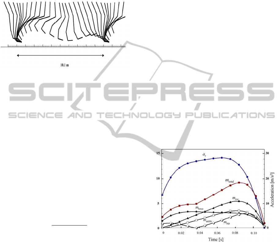
Figure 6: Stick diagram of the segment in running motion
at a speed of 14.1 m/s, as it appeared in the simulation.
The stride length is 10.1 m and the cyclic period is 0.716 s.
This is the fastest running speed that appeared in the
simulation with a moderate vertical acceleration of 28.3
m/s
2
.
Figure 6 shows a sample of the calculation from this
high-speed region with a velocity of 14.1 m/s and a
moderate vertical acceleration of 28.3 m/s
2
. The
running motion with a 14.1 m/s velocity is shown as
a stick diagram whose stride length is 10.1 m and
whose cyclic period is 0.716 s.
Faster running speeds show considerably larger
values for vertical acceleration; for example, a
velocity of 20 m/s leads to a vertical acceleration of
60 m/s
2
.
The required muscle mass m
i
of a 14.1 m/s
running speed during the stance phase is shown in
Fig. 6. m
i
represents the muscle mass fraction for the
i-th joint to the total body mass:
cos
100
(%)
body
crm
LdM
m
i
i
(6)
In Eq. (6), muscle density d = 1.06 × 10
3
kgm
−3
and
the fraction of active muscle volume c = 1 are
relatively reliable parameters. The total body mass
m
body
is not an intrinsic parameter because joint
moment M
i
includes the m
body
× (gravitational
acceleration) term, which leads to cancelation of the
factors. Although the expression does not contain a
total mass factor, the theory is intended to apply in
the case of T. rex with a total mass of 6 tons. The
estimation results in m
body
= 6071.82 kg for the
MOR 555 sample (Hutchinson et al., 2007).
L, r, and
θ
represent the muscle fiber length,
moment arm, and pennation angle of the muscle
fiber, respectively. The employed values for these
parameters are the same as those of previous works
(Hutchinson and Garcia, 2002; Hutchinson, 2004;
Gatesy et al., 2009).
σ represents the maximum muscle stress and
setting this value is a controversial problem. The
author’s future publication describes this parameter
in detail. For now, it is sufficient to say that the
reported value of
σappears to span as wide a range
as 11–220 N/cm
2
. This is probably because of
species’ adaptation of muscle ability. The reported
value of
σ is in the range of 11–90.3 N/cm
2
for the
human knee and ankle muscle groups. However, it is
noted that much of the data for
σ is located in the
range of 20–40 N/cm
2
. Thus, in this work, σis set as
30 N/cm
2
, which is the same as that of previous
works (Hutchinson and Garcia, 2002; Hutchinson,
2004; Gatesy et al., 2009).
Figure 7 shows the required muscle mass
fraction m
i
as it corresponds to the stance phase
shown in Fig. 6. It is observed that no value of m
i
exceeds 7%. Hutchinson states that if m
i
surpasses
7%, the bipedal animal is less likely to run quickly
(Hutchinson, 2004). Thus, the results of our
numerical simulations suggest the possibility that T.
rex could run quickly. The sum of m
i
,
i
mm
total
,
is also shown in Fig. 7.
Figure 7: Required muscle mass fraction m
i
for the i-th
segment of the leg in the stance phase shown in Fig. 6.
Black triangle, white square, black rhombus, and white
circle represent m
i
values for the toe, ankle, knee, and hip,
respectively. The vertical acceleration of the center of
mass is also shown as a black circle. In this case, the
maximum vertical acceleration is 28.3 m/s
2
, which yields a
maximum required muscle mass m
total
= 9.2%. Note that σ
is set as 30 N/cm
2
in this graph.
In Hutchinson’s work, m
i
of the toe joint is omitted
(Hutchinson, 2004) because the ankle extensors
could have produced most of the required toe joint
moments.
It is observed that the maximum value of m
total
is
Muscle mass m
i
[
%
]
APossibilityofFastRunningofTyrannosaurusrexbytheResultofEvolutionaryComputation
149
9.2%, yet computer-aided mass distribution analysis
reveals an m
total
of 14.2%–16.0% in other studies
(Bates et al., 2009; Hutchinson et al., 2007). Thus,
the result of even this criterion in the running
simulation suggests the possibility that T.rex could
run quickly.
If it is 36cm cranial that is a value obtained in the
work (Hutchinson et al., 2007), the value of
m
total
is
corrected as approximately twice larger one. A
detailed discussion on the problem of the center of
mass is given in forthcoming work (Usami, 2014).
The maximum value of vertical acceleration, as
shown in Fig. 7, is 28.3 m/s
2
. A vertical acceleration
of 18.3 m/s
2
(~1.87 × 9.8) is allowed in Gatesy et
al.’s estimation of static postures (Gatesy et al.,
2009); however, they also state, “In light of the large
number of options available to most theropods at
running GRFs of 2-4 BW (Body Weight), further
optimization analysis and consideration of the entire
stride cycle may reveal why specific poses are
chosen over so many alternatives.” This study’s
result of 29.3 m/s
2
(~3.0 BW) is within this range. In
addition, the entire stride cycle was obtained by
dynamical calculation with well-described
parameters. Thus, this work is a possible answer to
their unsolved question.
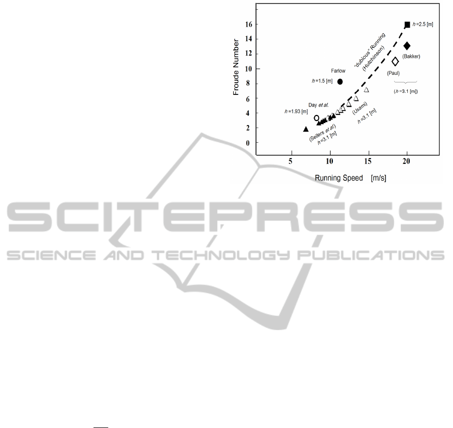
2.4 Comparison with Other Works
This section provides a detailed discussion on the
use of the Froude number to simulate a large,
bipedal dinosaur running. In our simulation, the
Froude number is calculated as Fr = 2.7–6.5 for a
running velocity v = 8.9–14.1 m/s. The Froude
number Fr is defined as
hg
v
Fr
2
,
(7)
where v, h, and g are the velocity, hip height, and
gravity constant, respectively. Our simulations are
shown as the white triangle in Fig. 8. The black
triangle shows Sellers et al.’s data as reported in
their Fig. 4 (Sellers and Manning, 2009). The black
square shows the data of Hutchinson and Garcia for
the case of h = 2.5 m (Hutchinson and Garcia, 2002).
From a fossilized footprint found in Texas,
U.S.A., Farlow reported a dinosaur trackway of L
st
=
6.59 m and a stride/hip height ratio of 4.3 (Farlow,
1981). From Farlow’s data, the hip height and
Froude number are calculated as h = 1.50 m and Fr
= 8.39, respectively.
Figure 8: Froude number vs. dinosaur running speed from
the literature and this study.
Day et al. reported a dinosaur trackway of L
st
= 5.65
m found in 163-million-year-old strata in the U.K
(Day et al., 2002) and reported an estimated hip
height of h = 1.93 m from the foot and a running
speed that might be v = 8.11 m/s. The corresponding
Froude number in this case is calculated as Fr = 3.5.
These observational data are shown as black and
white circles in Fig. 8.
In Fig. 8, black and white triangles show the
simulation results from Sellers and Manning (Sellers
and Manning, 2009) and this paper, respectively.
Note that Sellers and Manning presented data
requiring a muscle mass of 22.5% for Fr = 3.8 and a
running speed of 10.7 m/s. The black circle
represents Farlow’s data from the fossilized
footprint with a hip height of h = 1.5 m (Farlow,
1981). The white circle represents Day et al.’s data
from the footprint with a hip height of h = 1.93 m
(Day et al., 2002). The black and white rhombuses
are Bakker and Paul’s estimations for running
speeds of 20 m/s and 17.9 m/s, respectively, with an
assumption of h = 3.1 m; their running speeds are
based on the morphological consideration of muscle
and limb structure (Bakker, 1986; Paul, 1988).
Despite their different methodologies, all these
works state that T.rex would run at a speed of 7–20
m/s.
On the contrary, only works using the static
method state that T.rex would not be able to reach
speeds of 20 m/s (Hutchinson and Garcia, 2002). In
2004, Hutchinson stated, “speeds >11 m/s remain
dubious” (Hutchinson, 2004). The thick dashed
curve in Fig. 6 shows Hutchinson’s “dubious” range
(Hutchinson, 2004), whereas the black square
represents Fr = 16 with a running speed of 20 m/s
ECTA2014-InternationalConferenceonEvolutionaryComputationTheoryandApplications
150
and a hip height of h = 2.5 m, data from which
Hutchinson and Garcia claim no running could occur.
(Hutchinson and Garcia, 2002).
From the data, it seems that Hutchinson et al.’s
assumption of Fr = 16 would be a large value for T.
rex’s ability to run. However, note that speed
estimation using Froude number is qualitative and
has uncertainty in quantitative evaluation.
3 CONCLUSIONS
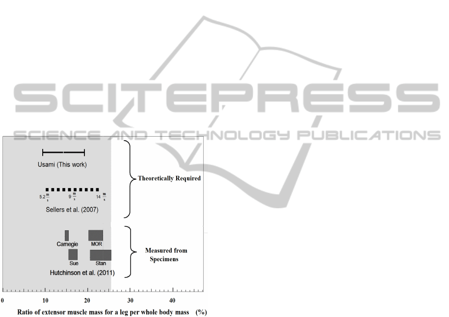
In 2011, Hutchinson et al. conducted 3D scanning of
four adult and one juvenile specimens of well-
preserved T.rex skeletons and analyzed their mass
distributions (Hutchinson et al., 2011). In particular,
remarkable from their report is an evaluation of the
amount of extensor muscle for a leg. Because
muscles are composed of extensor and flexor
muscles, the evaluation of the extensor muscle is a
monumental contribution to this field.
Figure 9: Ratio of extensor muscle mass for a leg per
whole body mass. The bottom four specimens are CM
9380 (Carnegie), FMNH PR 2081 (Sue), MOR 555
(MOR), and BHI 3033 (Stan) (Hutchinson et al., 2011).
The ratio of the extensor muscle mass relative to the
whole body mass is shown at the bottom of Fig. 9.
The upper three data in Fig. 9 show theoretically
required values of the ratio. Note that the most
probable body mass estimation of these four
specimens is in a range of 6000–9500 kg, which is
heavier than the one assumed in this paper based on
earlier studies. As seen from this graph, the
theoretically required and measured data overlap.
Thus, it cannot be said that T.rex could not run fast.
REFERENCES
Alexander, R. Mc. N., 1976. Estimates of speeds of
dinosaurs. Nature 261: 129-130.
Alexander, R. Mc. N. and Jayes, A. S., 1983. A dynamic
similarity hypothesis for the gaits of quadrupedal
mammals, J. Zool. 201: 135-152.
Alexander, R. Mc. N., 1989. The Dynamics of Dinosaurs
and Other Extinct Giants (Columbia University Press,
New York).
Alexander, R. Mc. N, 2006. Dinosaur biomechanics, Proc.
Roy. Soc. B 273: 1849-1855.
Bakker, R. T., 1986. Dinosaur Heresies (William Morrow,
New York).
Bates, K. T., Manning, P. L., Hodgetts, D. & Sellers, W. I.
Estimating Mass Properties of Dinosaurs Using Laser
Imaging and 3D Computer Modelling, PLoS ONE,
(2009) 4 (2): e4532 doi:10.1371/journal.pone.0004532.
Day, J. J., Norman, D. B., Upchurch, P. and Powell, H. P.,
2002. Dinosaur locomotion from a new trackway,
Nature 415: 494-495.
Farlow, J. O., 1981. Estimates of dinosaur speeds from a
new trackway site in Texas. Nature 294: 747-748.
Fogel, L. J., 1995. The Valuated State Space Approach
and Evolutionary Computation for Problem Solving,”
In Computational Intelligence: A Dynamic System
Perspective, edited by M Palaniswami, Y Attikiouzel,
RJ Marks, D Fogel, and T Fukuda, IEEE Press, NY, pp.
129-136.
Fraser, A. and Burnell, D., 1970. Computer Models in
Genetics. New York: McGraw-Hill.
Goldberg, D., 1989. Genetic Algorithms in Search,
Optimization and Machine Learning. Reading, MA:
Addison-Wesley Professional. ISBN 978-0201157673.
Gatesy, S. M., Baker, M. and Hutchinson, J. R., 2009.
Constraint-Based Exclusion of Limb Poses for
Reconstructing Theropod Dinosaur Locomotion. J.
Vert. Paleo 29: 535-544.
Hutchinson, J. R. and Garcia, M., 2002. Tyrannosaurus
was not a fast runner. Nature 415: 1018-1021.
Hutchinson, J. R., 2004. Biomechanical modeling and
sensitivity analyis of bipedal running ability. II. Extinct
taxa, J. Morph. 262: 441-461.
Hutchinson, J. R., Anderson, F. C., Blemker, S. S. and
Delp, S. L., 2005. Analysis of hindlimb muscle
moment arms in Tyrannosaurus rex using a three-
dimensional musculoskeletal computer model:
implications for stance, gait, and speed, Paleobiology
32: 676-701.
Hutchinson, J. R. Ng-Thow-Hing, V. and Anderson, F. C.
A 3D interactive method for estimating body
segmental parameters in animals: Application to the
turning and running performance of Tyrannosaurus
rex, J. Theor. Bio., (2007) 246: 660-680.
Hutchinson, J. R., Bates, K. T., Molnar, J., Allen, V. and
Makovicky, P. J., 2011. Computational analysis of
limb and body dimensions in Tyrannosaurus rex with
implications for locomotion, ontogeny, and growth,
PlosOne 6: e26037(1-20).
APossibilityofFastRunningofTyrannosaurusrexbytheResultofEvolutionaryComputation
151

Holland, J., 1992. Adaptation in Natural and Artificial
Systems. Cambridge, MA: MIT Press. ISBN 978-
0262581110.
Paul, G. S., 1988. Predatory Dinosaurs of the World
(Simon & Schuster, New York).
Usami, Y. and Kitaoka, M., 1997. Traveling salesman
problem and statistical physics, Intern. J. Modern
Phys., 11: 1519-1544.
Usami, Y. and Kano, Y., 1995. New method of solving the
traveling sales man problem based on real space
renormalization theory, Phys. Rev. Lett., 75: 1683-
1686.
Usami, Y., et al., Reconstruction of Extinct Animals in the
Computer”, Artificial Life VI, (C. Adamis, et al., eds.
MIT Press 1998). pp 173-177.
Usami, Y., 2014. Biomechanics of bipedal dinosaur: How
fast could Tyrannosaurus run? (to be published).
Sellers, W. I., Manning, P. L., Lyson, T., Stevens, K. and
Margetts, L., 2009. Virtual palaeontology: gait
reconstruction of extinct vertebrates using high
performance computing, Palaeontologia Electronica
12.3.13A: 1-14.
ECTA2014-InternationalConferenceonEvolutionaryComputationTheoryandApplications
152
