
Advanced Route Optimization in Ship Navigation
Ei-ichi Kobayashi, Syouta Yoneda and Atsushi Morita
Graduate School of Maritime Sciences, Kobe University, 5-1-1 Fukaeminami, Higashinadaku, Kobe, Japan
Keywords: Ship Weather Routing, Reducing Fuel Consumption, Weather Forecast, Ship Navigation Mathematical
Model.
Abstract: It is expected that international sea transportation will continue to increase as the world population
increases. The International Maritime Organization (IMO) requires preparation of ship navigation efficiency
management plans, including improvement in ship cruising methods such as appropriate ship trajectory
selection. Moreover, shipping companies pay careful attention to fuel consumption and environmental
conservation, while striving to maintain navigation safety and punctual cargo arrival. Generally speaking,
slow navigation results in energy savings, but takes longer. Ship speed is determined on the basis of such
factors as customer transportation-time and cost requirements, ship officers’ wages, insurance, port charges,
and ship building costs. Operational methods in ship navigation are limited to output reduction and route
selection. In this paper, we propose a newly developed weather routing optimization technology that
monitors fuel consumption, considering on-going sea and weather condition variation, including wind,
waves, and current.
1 INTRODUCTION
Weather routing is defined as selection of an optimal
sea route from one point to another point by
considering evaluation standards such as safety,
convenience, fuel consumption, minimum voyage
time considering ship conditions, and/or ability and
performance using estimated weather and sea
conditions. Seafarers have used wind, waves, and
current in voyages since ancient times, but as a
result of developments in weather forecast
technology, improvements in computer performance,
and establishment of physical mathematical dynamic
models in ship navigation, weather routing has
advanced substantially in recent times.
In 1957 R.W James tried to apply weather
forcast information to ship navigation from the
viewpoint of minimum voyage time using an
isochrone method(James, 1965). More recently,
many methods have been proposed considering not
only voyage time, but also fuel consumption and
CO
2
emissions.(Takashima, 2004)(Tsujimoto, 2005).
Moreover, since 2013 the International Maritime
Organization (IMO) has required ships of 400 gross
tonnage or more to prepare a Ship Energy Efficiency
Management Plan (SEEMP). This guideline includes
the weather routing method as one of the effective
measures for improving voyage efficiency.
In this paper, we propose a newly developed
weather routing optimization technology that treats
fuel consumption considering variation of on-going
sea and weather conditions such as wind, waves, and
current.
2 MATERIALS AND METHODS
2.1 Mathematical Model
A mathematical model for ship navigation consists
of three-dimensional independent free expressions,
such as surge, sway, and yaw motion, as in
differential equations that treat the dynamical
relationship between inertial forces and moment and
other hydrodynamic forces and moments of hull,
propeller, and rudder, as well as external forces and
moments. In these equations, steady forces acting on
a hull owing to wind, current, and added resistance
due to waves are taken into account as external
forces and moments. These equations in relation to
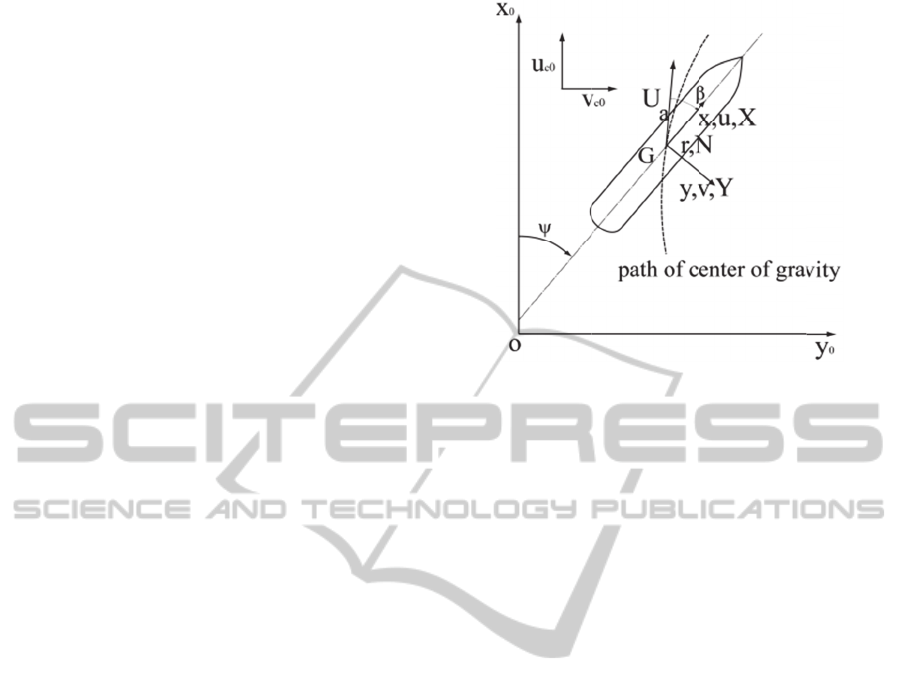
the coordinate system in Figure 1 are as follows:
572
Kobayashi E., Yoneda S. and Morita A..
Advanced Route Optimization in Ship Navigation.
DOI: 10.5220/0005033805720577
In Proceedings of the 4th International Conference on Simulation and Modeling Methodologies, Technologies and Applications (SIMULTECH-2014),
pages 572-577
ISBN: 978-989-758-038-3
Copyright
c
2014 SCITEPRESS (Science and Technology Publications, Lda.)
where
m
moment
the add
e
the add
e
the add
e
the z-a
x
directio
n
directio
n
are time
X
, Y
,
forces
a
respecti
v
lateral f
o
p
ropelle
r
longitud
i
acting o
are the
l
wind m
o
are the
respecti
v
and late
r
Represe
n
are sho
w
p
roporti
o
derived
f
In t
h
N
ationa
l
(NCEP)
while th
e
Oceanic
is dete
r
addition
,
and wa
v
the lates
ocean-g
o
4 indi
c
signific
a
current,
r
mm
u
X
X
X
mm
v
Y
Y
Y
I
N
N
N
m
is the mas
s
of inertia of
t
e
d mass of th
e
e
d mass of th
e
e
d mass mom
e
x
is, u is the
n
, v is the
v
n
, r is the turn
i
differentiati
o
and N
ar
e
and the m
o
v
ely, X
, Y
,
a
o
rces and the
m
r
s, respectiv
e
i
nal and lat
e
n the rudde
r
,
l
ongitudinal
a
o
men
t
, respe
c
longitudin
a
v
ely; and X
,
Y
r
al current for
c
n
tative expre
s
w
n in APPEN
D
o
nal value
t
f
rom equatio
n
h
is research
,
l
Center f
o
are used wit
h
e
five-day av
e
and Atmosp
r
mined with
,
in regard to
v
e data were
u
t forecast dat
a
o
ing navigati
o
c
ate the w
i
a
nt wave h
e
r
espectively,
o
u
mm
X
X
X
v
mm
Y
Y
Y
J
r
N
N
N
s
of the shi
p
t
he ship abou
t
e
ship in the
e
ship in the
e
nt of inertia
velocity co
m
v
elocity com
p
i
ng angular v
e
o
ns of u, v, a
n
e
the longit
u
o
ment actin
g
a
nd N
are th
e
m
oment acti
n
e
ly; X
, Y
,
e
ral forces
a
,
respectivel
y
a
nd lateral wi
n
c
tively; and
X
a
l and late
r
Y
, and N
a
r
c
es and mom
e
s
sions of for
c
D
IX. Fuel oil
t
o shaft hor
s
n
(9) in the A
p
,
hindcast
v
o
r Environ
m
h
respect to w
i
e
raged value
f
heric Admin
i
respect to
the actual na
v
u
pdated in the
a
every three
o
n simulation
.
i
nd directio
n
e
igh
t
, and f
i
o
n 25 Decem
b
vr
X
ur
Y
N
p
, I
is the
m
t
the z-axis,
m
x-direction,
m
y-direction;
J
of the ship a
b
m
ponent in th
e
p
onent in th
e
e
locity, u, v,
a
n
d
r
, respecti
v
u
dinal and la
t
g
on the
s
e
longitudina
l
n
g on the rota
t
and N
are
a
nd the mo
m
y
; X
, Y
, an
d
n
d forces an
d
X
, Y
, and
r
al wave f
o
e the longitu
d
e
n
t
, respectiv
e
c
es and mo
m
consumptio
n
s
e powe
r
(
S
p
pendix.
v
alues from
m
ental Predi
c
i
nd and wave
f
rom the
N
ati
i
stration (NO
A
current data
.
v
igation, the
w
calculation
u
hours in the
.
Figures 2, 3
n
and velo
i
ve-day aver
a
b
er 2009.
(1)
m
ass
m
is
m
y
is
J
zz
is
b
out
e x-
e
y-
a
nd r
v
ely,
teral
s
hip,
l
and
t
able
the
m
ent
d
N
d
the
N
o
rce,
d
inal
e
ly.
m
ents
n
is a
S
HP)
the
c
tion
data
i
onal
AA)
. In
w
ind
u
sing
ship
and
city,
a
ged
2.
2
Th
e
co
n
the
de
p
sol
v
co
n
des
sol
v
for
e
si
m
fro
m
ti
m
rev
i
fro
m
we
a
Po
w
me
t
der
i
thi
s
cal
c
the
cur
v
the
me
t
for
Bé
z
wo
r
is s
h
Fig
u
2
Route
O
e
route op
t
n
ducted
b
y
m
total fuel c
o
p
arture point
v
ing the abov
e
The total fu
e
n
ducting navi
g
tination
p
oi
n
v
ing equatio
n
e
cast. At a
m
ulation (for
e
m
the point c
o
e from the s
t
i
ewed using
a
m
the startin
g
a
ther routing
w
ell’s metho
d
t
hod that
d
i
vatives of a
n
s
study, Merc
c
ulations, suc
h
route is ex
p
v
e enabling
u
curve. The
t
hod is repla
c
expression o
f
z
ier curve is
d
rk
(Ishii, 2009
)
h
own in Figu
r
u
re 1: Coordin
a
O
ptimizati
o
i
mization i
n
m
inimizing a
c
o
nsumption i
n
to destinatio
n
e
-mentioned
e
e
l consumpti
o
g
ation from
t
along the
n
(1) under
t
particular n
a
e
xample, thre
e
o
rresponding
t
t
arting point
t
a
revised we
a
g
one. Repeat
i
problem is s
o
d
(Powell,1964
oes not re
q
n
objective
fu
ator sailing i
s
h
as distance
p
ressed using
u
s to generate
route optim
i
ed by findin
g
f
the Bézier
c
d
efine
d
as six
)
. This route
o
r
e 2.
a
te system.
o
n
n
this rese
a
c
ost function
n
the naviga
t
n
point, calc
u
e
quations.
on was calc
u
the start poi
n
designated
c
t
he star
t
-tim
e
a
vigation ti
m
e
hours later)
,
to the same
n
to the destin
a
a
ther forecast
i
ng this proc
e
o
lved iterati
v
4
), a conjugat
e
q
uire calcul
a
f
unction. Mo
r
s
used for sh
or course. In
a high-degr
e
e
the complex
i
zed using t
h
g
appropriate
c
urve. The or
d
based on ou
r
o
ptimization
p
a
rch was
deno
t
ing
t
ion from
u
lated by
u
lated by
n
t to the
c
ourse by
e
weather
m
e in the
,
a course
n
avigation
a
tion was
modified
e
dure, the
ely using
e
gradient
a
ting the
r
eover, in
i
p sailing
addition,
e
e Bézier
shape of
h
e Powel
valuables
d
er of the
r
previous
p
rocedure
AdvancedRouteOptimizationinShipNavigation
573
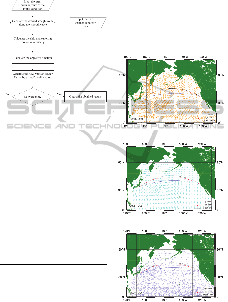
Figure 2: Flowchart of the proposed method.
First, the initial navigation route from start to
end is set. Next, a navigation simulation is
conducted by solving equation (1) from start to end
along the first navigation route, resulting in the
calculation of a cost function. Then, a new route
with a smaller cost function is found using Powell’s
method.
3 RESULTS AND DISCUSSION
Computer simulations were carried out for the
subject ship departing on 6 December 2008,
eastbound from Yokohama, Japan to San-Francisco,
U.S.A. to validate the efficiency of the proposed
method. A great circle route between Yokohama and
San Francisco was chosen for the iterative
calculation’s initial values, and a containership was
chosen as subject ship. The principal particulars are
shown in Table 1.
Table 1: Principal particulars of the subject ship.
Length 285.00 m
Breadth 40.00 m
Depth 24.30 m
Draft 14.02
An automatic rudder control algorithm was
introduced in this simulation for the ship to navigate
along the designated route as follows:
δ
∗
C
∆
y
C
∆ψC
r
(2)
where, δ
∗
,Δy,Δψ,andrare the command rudder
angle, lateral deviation from the route, deviation
from the designated course, and yaw rate,
respectively. In this formula, C
1
, C
2
, and C
3
are
empirical feedback gains. The propeller revolution
number was set to be constant through the
simulation.
Figures 3, 4, and 5 indicate the wind direction
and velocity, significant wave height, and five-day
averaged current prediction on 25 December 2009,
respectively.
Figure 3: Wind direction and speed at departure.
Figure 4: Significant wave height at departure.
Figure 5: Predicted ocean current at departure.
SIMULTECH2014-4thInternationalConferenceonSimulationandModelingMethodologies,Technologiesand
Applications
574
The above-mentioned figures denote the
predictions at the starting time. There are revised
predictions at times other than the starting time, such
as, for example, three hours later. Revised wave,
wind and current prediction data replaced previous
data in a navigation simulation from the starting
point to the destination.
Figure 6 shows the simulation results after
repeating this procedure, the east bound (red dotted
line) and west bound (blue dotted line) optimized
routes obtained using the above-mentioned method,
and the great circle route (black dotted line), the
initial route before the optimization.
Figure 6: Great circle and optimum fuel consumption
routes in the Pacific Ocean.
Both optimized routes are located south of the
great circle route, providing ships with fewer wind,
wave, and current effects.
Fuel oil consumption (FOC), voyage distance,
and voyage time are shown in Figures 7, 8 and 9.
Fuel oil consumption for the optimized routes are
2.0 tons and 24.9 tons less than the great circle route
Figure 7: FOC comparison with eastbound and westbound
routes.
Figure 8: Distance comparison with eastbound and
westbound routes.
Figure 9: Time comparison with eastbound and westbound
routes.
for the eastbound and westbound, respectively, and
travelling times are 0.1 hours and 2.3 hours shorter
than for the great circle, although distances are 3.8
miles and 57.2 miles longer than the great circle.
Thus, the optimized routes provide FOC savings and
travelling time reduction, although with increased
travelling distance.
4 CONCLUSIONS
An advanced new weather routing method for ship
navigation was proposed as a fuel oil consumption
minimization problem. The designated path is
expressed as a curve generated by a six-degree
Bézier curve, and the optimal route was calculated
by solving a cost function minimization using
Powell’s method. We found it possible to apply this
Eastbound Westbound
Great circle
1677,4 1752,2
Optimum
1675,4 1727,3
0
200
400
600
800
1000
1200
1400
1600
1800
2000
FOC[ton]
Eastbound Westbound
Great circle
4464,1 4464,9
Optimum
4467,9 4522,1
0
500
1000
1500
2000
2500
3000
3500
4000
4500
5000
Distance[mile]
Eastbound Westbound
Great circle
185,8 194,4
Optimum
185,7 191,9
0,0
50,0
100,0
150,0
200,0
250,0
Time[hour]
AdvancedRouteOptimizationinShipNavigation
575

method to the selection of an energy saving ship
navigation route in limited simulations.
Moreover, it is expected to develop and install a
new ship voyage on board instrument which
provides optimal ship navigation routes with help of
concurrent forecast of wind, wave and current
through, for example, satellite data communication
by applying this method.
On the other hand, there may exist a more
optimal path than this use of Powell’s method
provides, because the answer depends on the initial
conditions for the calculation. More work is required
to verify its applicability to determining actual
optimal routes.
ACKNOWLEDGEMENTS
The authors wish to thank Mr. Mizunoe and Ms.
Ishii and other students for their assistance in
completing the present study.
REFERENCES
Ishii, E., Kobayashi, E., 2010. Proposal of new-generation
route optimization technique for an oceangoing vessel,
Proceedings of OCEANS IEEE 2010, May 24-27,
Sydney.
James R. W., 1965. Application of wave forecasts to
marine navigation, U. S. Navy Hydrographic Office,
Washington, D.C..
Powell, M.J.D., 1964. An efficient method for finding the
minimum of a function of several variables without
calculating derivatives, The Computer Journal, vol.7,
no.2, pp. 155-162.
Takashima, K. Hagiwara, H., Shoji, R., 2004. Fuel saving
by weather routing–simulation using actual voyage
data of the container ship, The Journal of Japan
Institute of Navigation, vol. 111, pp. 259-266.
Tsujimoto, M., Tanizawa, K., 2005. Development of a
weather adaptive navigation system - influence of
weather forecast, Journal of the Japan Society of
Naval Architects and Ocean Engineers, vol.2, pp.75-
83.
APPENDIX
1
2
1
2
1
2
(3)
(4)
where
L,d
:
Length and depth of the ship
U
:
Speed of the ship(
√
)
У
:
Density of sea water
R
:
Ship resistance
1
0
0
(5)
where
X
,Y
,N
:
Forces and moment due to
propeller
1t
:
Thrust deduction factor
T
:
Thrust force by propeller
n
:
Revolution of propeller
:
Diameter of propeller
K
:
Coefficient of thrust force
:
Propeller advance constant
u
:
Inflow velocity to propeller
(6)
(7)
where
K
:
Coefficient of Torque
,
.
:
1.1.1.1 Coefficient from the
propeller characteristic curve
(8)
where
Q
:
Propeller torque
:
Density of sea water
SHP
2πn
(9)
SIMULTECH2014-4thInternationalConferenceonSimulationandModelingMethodologies,Technologiesand
Applications
576

2
where
SHP :
Shaft horse power
η
:
Transfer efficient
1
2
1
2
1
2
(10)
where
X
,Y
,N
: Wind forces and moment
ρ
: Density of air
θ
: Relative wind direction
V
: Relative wind speed [m/s]
: Transverse projected area
A
: Lateral projected area
C
,
,
: Wind force coefficients
∙0.51
.
∙
(11)
where
L
:
Length between perpendiculars
B
:
Breadth of the ship
:
Density of sea water
g :
Gravitation
F
:
Froude number
B
:
Bluntness coefficient
C
:
Prismatic coefficient
R
:
Additional resistance due to waves
H
:
Significant wave height
V
:
Speed of ship
AdvancedRouteOptimizationinShipNavigation
577
