
Evaluate Traffic Noise Level based on Traffic Microsimulation
Combined with a Refined Classic Noise Prediction Method
Chen Zhang
1
, Jie He
1
, Haifeng Wang
2
and Mark King
3
1
School of Transportation, Southeast University No.2, Sipailou, Nanjing 210096, China
2
School of Civil Engineering, Southeast University No.2, Sipailou, Nanjing 210096, China
3
Centre for Accident Research and Road Safety - Queensland, Queensland University of Technology
130 Victoria Park Rd, Kelvin Grove, QLD 4059, Australia
Keywords: Freeway, Road Widening, Traffic Microsimulation, Noise Prediction.
Abstract: In this paper, a refined classic noise prediction method based on the VISSIM and FHWA noise prediction
model is formulated to analyze the sound level contributed by traffic on the Nanjing Lukou airport
connecting freeway before and after widening. The aim of this research is to (i) assess the traffic noise
impact on the Nanjing University of Aeronautics and Astronautics (NUAA) campus before and after
freeway widening, (ii) compare the prediction results with field data to test the accuracy of this method, (iii)
analyze the relationship between traffic characteristics and sound level. The results indicate that the mean
difference between model predictions and field measurements is acceptable. The traffic composition impact
study indicates that buses (including mid-sized trucks) and heavy goods vehicles contribute a significant
proportion of total noise power despite their low traffic volume. In addition, speed analysis offers an
explanation for the minor differences in noise level across time periods. Future work will aim at reducing
model error, by focusing on noise barrier analysis using the FEM/BEM method and modifying the vehicle
noise emission equation by conducting field experimentation.
1 INTRODUCTION
As a result of rapid economic development of in
developing countries such as China, freeways and
motorways are being widened in many rural areas,
contributing to noise pollution in the vicinity of the
road. The variation in traffic flow rate and speed
before and after widening strongly influences the
emission of traffic noise, and single vehicle speed is
largely dependent on single vehicle dynamics
induced by a vehicle interactions model. Thus in
order to improve traffic noise estimation for freeway
widening, an accurate car following model and a
precise noise estimation model must be used to
analyze the interaction between traffic
characteristics and noise emission.
In the classic static traffic noise prediction
model, roads are divided into basic sections where
the traffic characteristics are considered smooth and
homogeneous. Examples of such models are the US
Federal Highway Administration model (FHWA
1978), the German RLS90 model (Steele C. 2001),
and other models which refine the emission law to
reveal different driving conditions, like the Nordic
model (Leclercq. 2001) and the ASJ RTN
Model(Yoshihisa et al. 2004).
To increase the accuracy of noise prediction,
some analytic models modify the vehicle speed
calculation algorithm in the static models. Each
subdivided segment in those models is no longer
speed-homogeneous; the speed-variation pattern for
a single isolated vehicle must be captured to attain
the mean speed profile, while the average speed is
needed to determine the acoustical energy at the
receiver from the traffic on the related roadway
sub-segment. Analytic models are often used as
some national standards, such as the US Federal
Highway Administration’s TNM model (Christopher
W. Menger et al. 1998) and the French noise
estimation model (A. Can et al. 2010). The progress
analytic models make lies in the fact that they
attempt to account for single vehicle dynamics,
although the TNM model only calculates the
entrance and exit speed and converts them to the
693
Zhang C., He J., Wang H. and King M..
Evaluate Traffic Noise Level based on Traffic Microsimulation Combined with a Refined Classic Noise Prediction Method.
DOI: 10.5220/0005035606930700
In Proceedings of the 4th International Conference on Simulation and Modeling Methodologies, Technologies and Applications (SIMULTECH-2014),
pages 693-700
ISBN: 978-989-758-038-3
Copyright
c
2014 SCITEPRESS (Science and Technology Publications, Lda.)

segment average speed (Arnaud Can et al. 2008).
This analytic model is suitable in the freeway
scenario, which has relatively continuous traffic
flow and less traffic characteristic variation.
In recent years, many researchers have focused on
dynamic models (Ruffin Makarewicz et al. 2011),
which can output not only hourly equivalent sound
level, but also instantaneous noise emission.
Dynamic models such as MOBILEE and
ROTRANOMO (Volkmar, H. 2005) are based on
different microsimulation methods, which can give
position, speed and acceleration of each vehicle.
When the values of these variables are substituted
into a noise emission law and sound propagation
algorithm, instantaneous sound pressure can be
calculated. Microsimulation models are well suited
for complex traffic situations such as cross
intersections and roundabouts, where traffic
characteristics are quite variable. However the
massive amounts of data involved necessitate large
amounts of computing power and calculation time.
This paper offers a refined classic noise
prediction method (analytic model) based on the
classic FHWA noise prediction model and using the
VISSIM traffic microsimulator to analyze the sound
level contributed by the traffic on the Nanjing Lukou
airport connecting freeway before and after its
widening. The aim of this research is to (i) assess the
traffic noise impact on the Nanjing University of
Aeronautics and Astronautics (NUAA) campus
before and after freeway widening, (ii) compare the
prediction results with the field data to test the
accuracy of this method, and (iii) analyze the
relationship between traffic characteristics and
sound level.
The organization of this paper is as follows: (i)
the first part describes the geometric layout of the
experimentation site, then discusses the traffic
microsimulation and noise prediction model
selected, and (ii) the second part demonstrates the
results and analyzes different traffic characteristics
and their impact on noise level.
2 METHODOLOGY
2.1 Case Study
2.1.1 Geometric Design
The selected study site is located on the Nanjing
airport connecting freeway, in a suburban district of
the city. It contains three lanes in the North to South
direction as well as in the opposite direction before
widening (current scenario). After widening, lane
number will be doubled in each direction, with the
new lanes being located in the middle of the origin
site (space was pre-reserved). The detailed
geometric design is shown in Figure1: (i) the overall
length of the studied freeway section is 400m,
including a 3.5m high barrier on the side where
noise levels are of interest; (ii) the width of the
traffic lanes is 3.75m, while the shoulder width is
3.3m; (iii) the tree zones after widening have two
different widths: 2.7m and 6.5m.
2.1.2 Field Data Collection
The experiment included traffic and acoustic
measurements, which were carried out before the
widening in two one-hour periods (7:30-8:30,
9:30-10:30) on a weekday. The two time periods
cover peak and normal traffic flows respectively.
The recorded traffic accounts for all traffic flow in
the freeway section as there are no access ramps or
intersections. Overall peak hour traffic flow
(7:30-8:30) was 6401 veh/h, comprised of 3376
veh/h in the north to south direction and 3025 veh/h
in the opposite direction. Normal traffic flow was
4833 veh/h, comprised of 2579 veh/h travelling
north to south and 2254 veh/h travelling in the other
direction. Three vehicle categories were recorded:
cars (including light trucks), heavy goods vehicles,
and buses (including mid-size trucks). The detailed
traffic composition is given in Table 1.
Acoustic recordings are L
,
(A-weighted
equivalent sound level for 1 second) for the points
P1, P2 (Figure 1) selected for sound pressure level
estimation. P1 was near the NUAA gym, and P2 was
in front of the student dormitory. Both were in the
barrier-contained section at the same cross section,
with receivers set 1.5m high.
2.2 Traffic Microsimulation
In this paper, the chosen traffic microsimulator
VISSIM (PTV. Ltd. 2007) was used to refine
dynamic speed calculation of the FHWA noise
prediction model. VISSIM is a microscopic, time
step and behavior based simulation model developed
to be applied in a variety of transportation problem
settings. The essential elements of traffic modeling
is the car following and lane change model which
directly affects vehicle interaction, especially
SIMULTECH2014-4thInternationalConferenceonSimulationandModelingMethodologies,Technologiesand
Applications
694
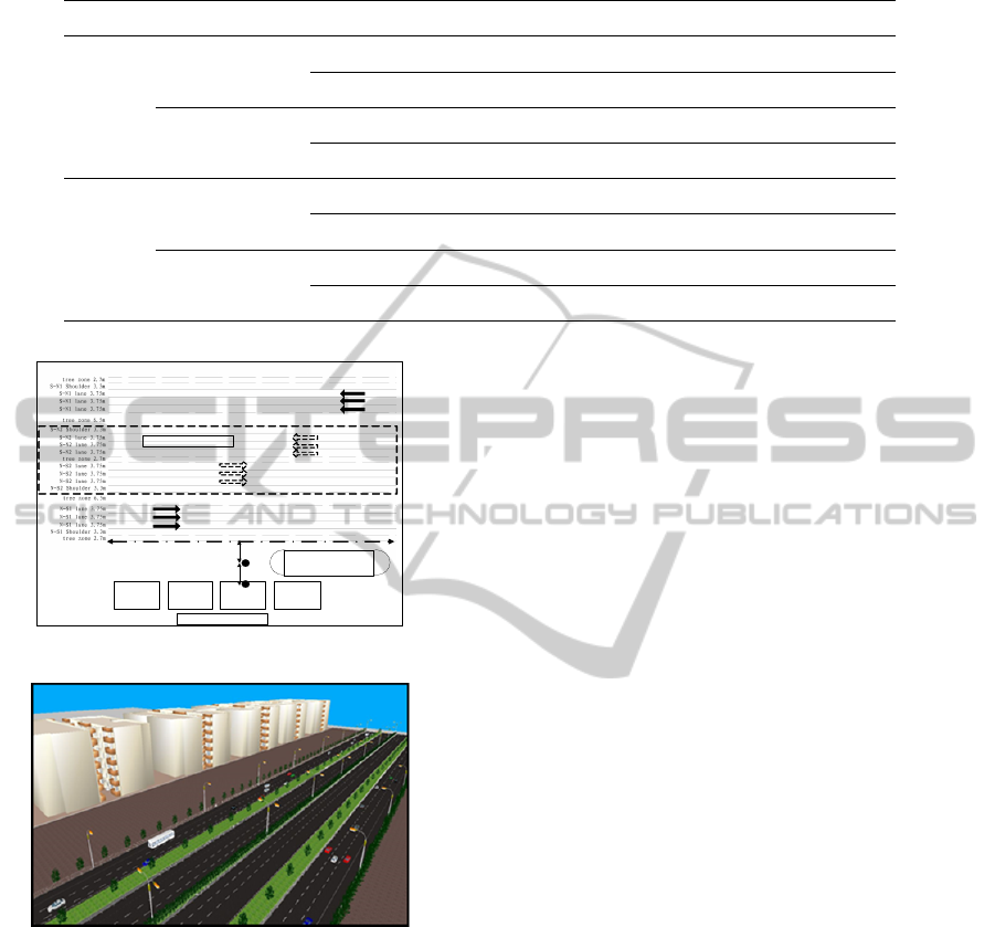
Table 1: Traffic composition (Before widening) (veh/h).
Time Direction Cars(LT) Bus(MT) HGV Total
Peak
North-South
(composition)
3114 169 93 3376
0.922 0.050 0.028 1.000
South-North
(composition)
2852 107 66 3025
0.943 0.035 0.022 1.000
normal
North-South
(composition)
2434 61 84 2579
0.944 0.023 0.033 1.000
South-North
(composition)
2101 65 88 2254
0.932 0.029 0.039 1.000
After widening
Student dormitory
gym
P1
P2
18m
22m
barriers
(a) 2D-view
(b) 3D-view
Figure 1: Geometric design.
dynamic speed at different cross sections. Thus we
used a psycho-physical car following model based
on the work of Wiedemann (PTV. Ltd. 2007).
(i) Input the traffic composition figures collected
from the field experiment before the freeway
widening and later input the assumed data after
widening, in order to analyze the impact of
widening on noise level.
(ii) Select the appropriate speeds for all the vehicle
types based on the field observations and
empirical data from Chinese freeways. The
speeds set for Car (LT), Bus (MT) and HGV
were respectively 90km/h, 70km/h, and
60km/h (For convenience, the speeds are set to
integer based on the observations).
(iii) Set the data collector at selected cross section
to collect instantaneous speed information.
Dynamic speed was used to calculate vehicle
noise emission and traffic adjustments (see
next section) for the noise prediction model.
2.3 Noise Level Estimation Process
The selected Federal Highway Administration
Traffic Noise Model (FHWA) predicts sound level
by adding a series of adjustments to a reference
noise level. It can also be used to aid in the design of
highway noise barriers. The FHWA model
calculation process includes vehicle noise emission
and noise propagation estimation. The general sound
level calculation is as follows:
2.3.1 Vehicle Noise Emission
The FHWA model contains noise-emission
equations for the five built-in vehicle types, but in
order to reduce complexity the medium trucks and
buses are regarded as Bus (MT) for convenience and
to be consistent with the vehicle type split in
VISSIM.
The vehicle noise emission calculation is based
on the FHWA noise emission database (Christopher
W. Menger et al. 1998). The maximum A-weighted
reference sound level as a single vehicle passes by a
receiver 15 meters to the side and 1.5m high is
considered to represent the entire vehicle’s
noise-emission level. For each vehicle type defined
above for use in VISSIM, the emission level is:
EvaluateTrafficNoiseLevelbasedonTrafficMicrosimulationCombinedwithaRefinedClassicNoisePredictionMethod
695

10
38.1log -2.4(dBA)
ocar car
LS
(1)
(MT) 10 (MT)
33.9 log +16.4(dBA)
obus bus
LS
(2)
010
24.6 log +38.5(dBA)
HGV HGV
LS
(3)
Si represents the average speed of each vehicle
type.
2.3.2 Traffic and Distance Adjustment for
Free Field Conditions
Free field sound conditions are first assumed, such
that the sound is assumed to travel without
boundaries (the effects of a barrier are addressed in
the next section). Based on the basic assumption that
the A-weighted reference sound level reaches its
peak value when a vehicle passes by the location
perpendicular to the receiver, we can derive a single
car’s free field noise level at any time by considering
only the distance attenuation:
2
0
010010
2
2
0
-20log = -20log (dBA)
+
t
RD
LL L
D
Dst
(4)
Where
s
t
refers to the distance a single car
travels during time period
t
,
D
refers to the
distance between the car and the receiver.
And for a continuous time period
12
~tt
(usually
1h), the equivalent sound level is:
2
1
2
1
10
10
21
2
0
010
2
2
1
10log 10 dt
-
1
= +10 log dt(dBA)
+
t
t
L
Aeq
t
t
t
LT
tt
D
L
T
Dst
(5)
For convenience, it is assumed that the short time
period during which a car passes by the receiver
contributes the greatest proportion of sound energy,
thus the equation can be rewritten:
2
+
0
010
2
2
-
00
010 10
1
+10 log dt
+
+10log +10log (dBA)
Aeq
LT
D
L
T
Dst
DD
L
sT D
(6)
Thus, given traffic volume
i
N
for each vehicle type
i
:
,
,
0
10
,10
=1
00
10
10
=1
10log 10
1
=10log 10 (dBA)
ij
Aeq
ij
j
N
LT
Aeq i j
j
N
L
j
ij
LNT
DD
NsTD
(7)
Note that in the classic FHWA model, the vehicle
speed for a single car of a specified type is always
defined as a constant value, which does not reflect
reality. Thus to improve the accuracy of the noise
level calculation, the data collector at the studied
cross section collected the instantaneous speed
profile, and with VB programming the hourly
equivalent free field sound level for each vehicle
type can be calculated.
2.3.3 Barrier Insertion Loss
Barriers are structures that are fixed vertically and
have a height and a base. The barrier insertion loss
estimation algorithm is based upon the Fresnel
diffraction theory, as described by De Jong,
Moerkerken, and Van der Toorn (Christopher W.
Menger et al.1998).
In the general scenario, barriers have diffracting
points at the bottom of the left face, the top, and the
bottom of the right face and for simplicity, a sound
barrier is usually defined as a thin material of a
particular height. The insertion loss equation for
sound barriers can be defined as follows:
10
123
111
=-10log + + (dBA)
3+20 3+20 3+20
bar
A
NNN
(8)
i
N
refers to the Fresnel number which can be
calculated from the equation
=2
ii
N
,
i
refers to
three kinds of sound propagation path differences
respectively , which are defined at the top, bottom
left and right face diffracting points.
is sound
wavelength computed from the center frequency 500
HZ for traffic and sound speed 340 m/s.
At the studied site, the sound barrier between the
receiver and the traffic is relatively infinite (the total
barrier length is approximately thousands of meters),
thus the attenuation equation can be simplified as
follows:
10
1
1
=-10 log (dBA)
3+20
bar
A
N
(9)
The diffracting points at the bottom of the right and
left face are irrelevant due to the barriers’ “infinite”
SIMULTECH2014-4thInternationalConferenceonSimulationandModelingMethodologies,Technologiesand
Applications
696

length.
2.3.4 Hourly Equivalent a-weighted Sound
Level for a Receiver
By adding the insertion loss to equation (Kurze U.J
et al. 1971), for a particular vehicle type, the hourly
equivalent A-weighted sound level for a receiver is:
,
0
,
00
10
10
=1
10
1
1
=10log 10
1
-10log (dBA)
3+20
ij
j
Aeq i j bar
N
L
j
ij
LNTA
DD
NsTD
N
(10)
Considering three input vehicle types and traffic
composition collected from field data or assumed
ones, the equation for overall noise level before and
after widening will be:
,,
,
10
10
10 log 10 10
10
,, ,T
=10log 10 (dBA)
LNTA
Aeq i j bar
i
Aeq bar
alldirectioin
L N T A otal
(11)
3 RESULTS
3.1 Model Verification
This part of paper provides a comparison of refined
FHWA model with field measurements in order to
evaluate the accuracy of the model. The comparisons
are made at two different selected points which are
set to evaluate the noise impact on the campus. The
hourly equivalent A-weighted noise level is
computed based on the VB (Microsoft Visual Basic)
programming using the instantaneous speed profile
generated by VISSIM simulation. The field
measurements
,1Aeq h
L
can be obtained from the
statistic noise levels
90
L
and
10
L
, which are derived
from initial collected descriptor
,1Aeq s
L
. The results
before the widening are shown in Table 2.
As can be seen in Table 2, both the prediction
results and field data exceed the recommended
standard of noise level in China (the accepted level
on campus is 55dBA), even before the impact of
widening is taken into account. The refined model
gives estimates that are on average 2.6 dBA higher
than the field results, an apparent improvement on
noise estimation using the classic model (usually a 3
dBA or more mean error is accepted). The reasons
for the overestimation could include: (i) the
application of the American standard to the current
scenario, (ii) elimination of ground attenuation,
which is hard to assess because of the geometric
complexity, (iii) simplification of the distance
between vehicle and receiver in the calculation to
compute
,Aeq i j bar
LNTA
using the VB program, or
(iv) underestimation of the effect of the noise barrier
by using a less complicated algorithm.
3.2 Traffic Composition Impact
Although the Car (LT) category contributes the most
sound energy for all time and direction combinations,
it is unwise to conclude that buses (MT) and HGV
have a minor impact on the noise level without also
considering the traffic flow for each type. For
example, the traffic flow for cars in the North to
South direction is 3114 veh/h, which contributes
60.7 dBA at receiver P1, while the HGV flow of
only 93 veh/h adds 57.2 dBA to the total sound level,
which is only 2.5 dBA less than car contribution,.
Thus, despite the relatively higher traffic attenuation
(adjustment) for Bus (MT) and HGV, their
contribution to overall noise cannot be ignored.
Figure 2 shows the selected traffic flow for each
type of vehicle and their related
,Aeq i j bar
LNTA
.
Table 2: Noise level comparison of refined model with field measurements (dBA).
Receiver Time period
Sum
(direction)
Field
data
P1
Peak 64.3 61.6
Normal 63.3 60.5
P2
Peak 62.2 59.8
Normal 61.5 58.9
EvaluateTrafficNoiseLevelbasedonTrafficMicrosimulationCombinedwithaRefinedClassicNoisePredictionMethod
697
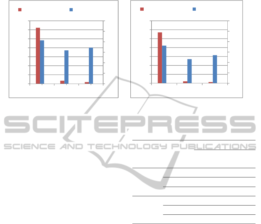
(a) North to South, peak hour, P1 (b) South to North, peak hour, P1
Figure 2: Selected traffic flow and noise contribution for each vehicle type.
3.3 Speed Analysis
Speed is also an important factor in analyzing the
traffic and noise level. As discussed above, the
speed profile generated by the VISSIM simulation
result was used to calculate the vehicle noise
emission and traffic adjustment for free field
conditions. The instantaneous speed of every vehicle
passing by the collector was extracted to estimate
the average speed for each direction and time period.
The results show a small increase in speed for cars
from peak to normal flow. For instance, the average
car speed in peak hour in the North to South
direction was 94.1 km/h, while in a normal hour for
the same direction, the speed increased to 95.4 km/h.
The fact that this increase is relatively low, in spite
of the decrease in traffic flow, suggests that the
freeway is far from over-saturated during peak hour.
Thus, combined with the fact the HGV category
contributes a lot to the noise level (and, as shown in
Table 1, the amount of HGV does not vary much
during different hours), suggests that the minor
difference in sound level between peak and normal
hours may be accounted for by the modest increase
in speed being insufficient to fully offset the noise
reduction due to the drop in traffic flow.
3.4 Noise Level Prediction after
Widening
After the widening of the freeway, the lane number
for each direction will double. The new lanes will be
located in the middle of the original lanes as shown
in Figure 1. Due to the lack of estimates of traffic
Table 3: Average speed for different time period before
widening.
Direction
Vehicle
type
Vehicle speed (km/h)
Peak hour
Normal
hour
North to
South
Car(LT) 94.1 95.4
Bus(MT) 72.7 73.1
HGV 63.0 62.6
South to
North
Car(LT) 94.2 95.5
Bus(MT) 72.8 72.7
HGV 63.5 63.7
flow after widening, this paper considers three
scenarios regarding possible vehicle numbers during
each split time period: (i) the traffic flow in each
direction remains the same, (ii) the traffic flow
increases by 50%, (iii) the traffic flow doubles. For
convenience, it is assumed that the traffic
composition (vehicle proportion) remains the same
and that half of the traffic flow takes place in the
new lanes for each scenario. Note that a scenario
involving a decrease in traffic has not been included
as it is considered highly unlikely. The calculation
results are shown in Figure 3.
The noise level of the first scenario drops slightly
despite traffic flow being the same as before
widening, after which noise level increases at a high
rate with increasing traffic, such that a 50% growth
in traffic is associated with approximate 1.2-1.5 dBA
increase in noise level. Thus, given that there is
already an unacceptable noise level at the campus
40
45
50
55
60
65
70
0
500
1000
1500
2000
2500
3000
3500
Car(LT) Bus(MT) HGV
trafficflow(Veh/h) noiselevel(dBA)
40
45
50
55
60
65
70
0
500
1000
1500
2000
2500
3000
3500
Car(LT) Bus(MT) HGV
trafficflow(Veh/h) noiselevel(dBA)
SIMULTECH2014-4thInternationalConferenceonSimulationandModelingMethodologies,Technologiesand
Applications
698
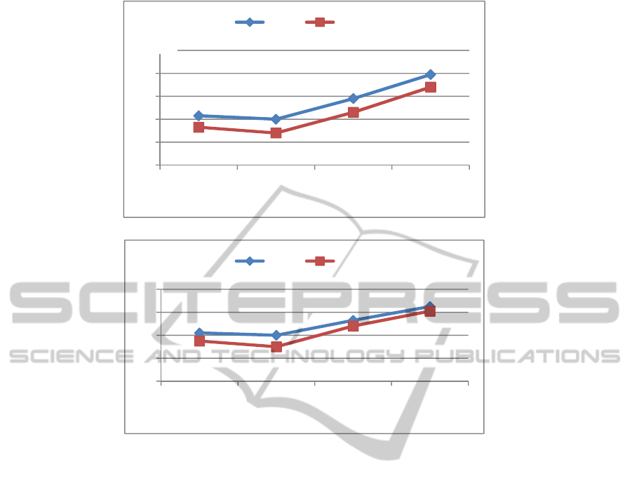
(a) Noise level at P1
(b) Noise level at P2
Figure 3: Noise level at receivers based on the three traffic flow scenarios.
under current conditions, the simple conclusion can
be drawn that, assuming that the widening will
attract higher levels of traffic, noise pollution on
campus will be worse than at present. This suggests
that consideration should be given to providing
additional noise barriers in the freeway section
adjacent to the campus.
4 CONCLUSIONS
In this paper, the author provides a refined classic
noise prediction model to estimate the noise level in
the campus of NUAA, which is caused by the traffic
in the Nanjing airport connecting freeway. The
refined method consists of a traffic microsimulation
and a classic noise estimation model, and VISSIM is
used to simulate the dynamic vehicle operation
condition (especially speed) to refine the noise
calculation process in the selected noise prediction
model. After thorough analysis of the estimation
results and traffic characteristics, conclusions can be
drawn as follows:
(i)
Sound levels predicted by the model exceed
field measurements by a more or less
acceptable level (2.6 dBA). The error could be
reduced by refining the vehicle emission level
assumptions, considering the ground diffraction
and reflection effect, and using a more complex
method to evaluate the sound barrier
attenuation (BEM/FEM methodology).
(ii)
Although they have a much lower traffic
volume than the Car (LT) category, the Bus
(MT) and HGV categories contribute
significant amounts of sound power which
should not be ignored. In addition, the
relatively low increase in speeds in the normal
traffic flow period explains why the increase in
noise due to the higher speed is largely offset
by the decrease in traffic flow.
64,3
64
65,8
67,9
63,3
62,8
64,6
66,8
60
62
64
66
68
70
before
widening
scenario(i) scenario(ii) scenario(iii)
peak normal
62,2
62
63,3
64,5
61,5
61
62,8
64,1
58
60
62
64
66
before
widening
scenario(i) scenario(ii) scenario(iii)
peak normal
dBA
dBA
EvaluateTrafficNoiseLevelbasedonTrafficMicrosimulationCombinedwithaRefinedClassicNoisePredictionMethod
699

REFERENCES
Steele C. A critical review of some traffic noise prediction
models. Journal of Applied Acoustics, 2001. Vol.
62(33): 271-287.
FHWA. Traffic noise prediction model. Washington:
Department of Transportation, Federal Highway
Administration National Technical Information
Service, 1978.
Arnaud Can, Ludovic Leclercq, et al. Accounting for
traffic dynamics improves noise assessment:
Experimental evidence. Journal of Applied Acoustics,
2008, (70): 821-829.
E. Chevallier, A. Can, et al. Improving assessment at
intersections by modeling traffic dynamics. Journal of
Transportation Research Part D, 2009 14: 100-110.
Ruffin Makarewicz, Michal Galuszka. Road Traffic noise
prediction based on speed-flow diagram. Journal of
Applied Acoustics, 2011 vol. 72 (4): 190-195.
A. Can, L. Leclercq, et al. Traffic noise spectrum analysis:
Dynamic modeling vs. experimental observations.
Journal of Applied Acoustics, 2010, vol. 71 (8):
764-770.
Kurze U. J, Aderson G. S. Sound Attenuation by Barrier.
Journal of Applied Acoustics, 1971, 4: 35-53.
Yamamoto K, Yoshihisa K, Miyake T, Tajika T,
Tachibana H. Road traffic noise prediction model
“ASJTN-model 2003” proposed by the Acoustical
Society of Japan-Part 3: Calculation model of sound
propagation [C]. In: Proceedings of the 18th
international congress acoustics, Kyoto, April, 2004,
(6): 2797-2800.
Christopher W. Menger, Christopher F. Rossano, Grant S.
Anderson, Christopher J, Bajdek. FHWA TRAFFIC
NOISE MODEL (FHWA TNW 1.0). Technical
Manual. Research Report. Publication No.
DOT-VNTSC-FHWA-98-2.1998.2.
PTV. Ltd. VISSIM 4.30 User Manual. 2007.
Leclercq. Dynamic evaluation of urban traffic noise. In:
Proceedings of the 17th International Congress on
Acoustics. 2001. Rome.
Volkmar, H. 2005. Development of a microscopic road
traffic noise model for the assessment of noise
reduction measures. In: Final Conference, Berlin,
<www.rotranomo.com>.
SIMULTECH2014-4thInternationalConferenceonSimulationandModelingMethodologies,Technologiesand
Applications
700
