Model Predictive Control for Fractional-order System
A Modeling and Approximation Based Analysis
Mandar M. Joshi
1
, Vishwesh A. Vyawahare
2
and Mukesh D. Patil
2
1
Department of Electrical Engineering, Government College of Engineering, Pune, India
2
Department of Electronics Engineering, Ramrao Adik Institute of Technology, Nerul, Navi Mumbai, India
Keywords:
Predictive Control, Fractional Calculus, Fractional Systems, Integer-order Approximation, Internal Model
Control.
Abstract:
A widely recognized advanced control methodology model predictive control is applied to solve a classical
servo problem in the context of linear fractional-order (FO) system with the help of an approximation method.
In model predictive control, a finite horizon optimal control problem is solved at each sampling instant to
obtain the current control action. The optimization delivers an optimal control sequence and the first control
thus obtained is applied to the plant. An important constituent of this type of control is the accuracy of the
model. For a system with fractional dynamics, accurate model can be obtained using fractional calculus. One
of the methods to implement such a model for control purpose is Oustaloup’s recursive approximation. This
method delivers equivalent integer-order transfer function for a fractional-order system, which is then utilized
as an internal model in model predictive control. Analytically calculated output equation for FO system has
been utilized to represent process model to make simulations look more realistic by considering current and
initial states in process model. The paper attempts to present the effect of modeling and approximations of
fractional-order system on the performance of model predictive control strategy.
1 INTRODUCTION
Model predictive control (MPC) is an optimal control
theory based on numerical optimization. Future con-
trol efforts and future plant responses are predicted
using a system model and optimized at regular in-
tervals with respect to a performance index. It is a
computational technique for improving control per-
formance in applications and processes in chemical
and petrochemical industries. Predictive control has
become arguably the most widespread advanced con-
trol methodology currently in use in industry (Muske
and Rawlings, 1993; Rawlings, 2000; Morari and
Lee, 1999; Bemporad, 2006; Garcia et al., 1989).
The basic MPC concept can be explained as fol-
lows. In MPC, model of the system is used to pre-
dict the future output and control efforts required to
attain the reference trajectory. Hence, the accuracy
of the model determines the control and delivers pre-
cise future input trajectory in order to follow the refer-
ence signal. This is the basic philosophy of any MPC.
MPC is more a methodology and not a single tech-
nique and it is known by many different nomencla-
tures such as Model Predictive Control (MPC), Model
based predictive control (MBPC), Receding horizon
control (RHC), Moving horizon control (MHC), In-
ternal Model Control (IMC) etc.
The literature survey reveals that MPC has made
outstanding contributions for solving control prob-
lems in industry (J.M.Maciejowski, ). It has so far
been applied mainly in the petrochemical industry, but
is currently being increasingly applied in other sectors
of the process industry. The main advantages of using
MPC in these applications are:
1. Inherent handling of multivariable control prob-
lems.
2. Actuator limitations are considered.
3. Operation closer to constraints is possible for
more profitability.
4. Applications with relatively low control update
rates provides sufficient time for the necessary on-
line computations.
Fractional calculus is used for modeling real-world
and man-made systems more compactly and faith-
fully. Fractional calculus has been known from
1695, when Leibnitz introduced the symbol for the
n
th
derivative d
n
y/dx
n
, and L’Hopital discussed the
361
Joshi M., Vyawahare V. and Patil M..
Model Predictive Control for Fractional-order System - A Modeling and Approximation Based Analysis.
DOI: 10.5220/0005038203610372
In Proceedings of the 4th International Conference on Simulation and Modeling Methodologies, Technologies and Applications (SIMULTECH-2014),
pages 361-372
ISBN: 978-989-758-038-3
Copyright
c
 2014 SCITEPRESS (Science and Technology Publications, Lda.)

possibility that ‘n’ could be 1/2. Nonetheless, this
branch of mathematical analysis was really developed
in the 19
th
century by Liouville, Riemann, Letnikov
and others (Monje et al., 2010). One of the most
popular examples of fractional-order modeling of a
physical system is the semi-infinite lossy transmission
line (Boudjehem and Boudjehem, 2012). Other sys-
tems with fractional-order dynamics are viscoelastic-
ity, dielectric polarization and electromagnetic waves
(Boudjehem and Boudjehem, 2012). Fractional-order
control can be regarded as the generalization of the
conventional integer-order control theory. Fractional-
order models represent a system in more accurate
ways (Boudjehem and Boudjehem, 2012). It is
worth exploring the introduction of fractional theory
in MPC. There are some systems which are of frac-
tional nature and hence a fractional-order model can
be used to represent such systems instead of integer-
order models.
For implementation of MPC, a state-space model
is required and approximation method helps to ob-
tain the same. A fractional-order Transfer Function
(FOTF) can not be converted to a state-space model
through simulation softwares like MATLAB. There-
fore, we need to get an approximation that is, an
integer-order equivalent (transfer function) which can
represent that FOTF and also can be converted to
state-space model using MATLAB. Moreover, an ap-
proximation has to be made for a fractional operator
s
α
or s
−α
with 0 < α < 1.
In this paper,MPC is applied to an FO system with
different fractional-order α for which Oustaloup’s re-
cursive approximation has been used to obtain re-
spective models. Obtained models are then converted
to acquire strictly proper natured discrete state-space
models by adding a pole at far away from the origin.
Authenticity of these models were checked with the
original one through frequency and step response. Fi-
nally, these models were used for prediction purposes
in MPC. In order to make MPC realistic, analytically
calculated output equation for FO systems has been
utilized to represent process output.
The paper is organized as follows. In Section
2, definition of fractional calculus and dynamics of
FO systems are reviewed; Section 3 presents the
Oustaloup’s recursive approximation method and its
application for fractional operators. Philosophy be-
hind MPC and formulation of MPC problem is cov-
ered in section 4. Section 5 presents the results ob-
tained for MPC with FO systems and section 6 con-
cludes this work with some observations.
2 FRACTIONAL CALCULUS
Fractional Calculus can be defined as integration and
differentiation of non-integer order. In the develop-
ment of the theory of fractional calculus, there are dif-
ferent definitions available for fractional-order inte-
gration and differentiation such as Riemann-Liouville
fractional differentiation and integration, Caputo frac-
tional differentiation, Grunwald-Letnikov fractional
differentiation (YaLi and Ruikun, 2010). Caputo frac-
tional differentiation is defined as (Podlubny, 1998)
C
0
D
α
t
f(t) =
1
Γ(m−α)
Z
t
0
(t − τ)
(m−α−1)
D
m
τ
f(τ)dτ,
(1)
where α is the order of the differentiation and m is the
nearest integer on higher side of α.
2.1 Fractional-order Systems
Fractional-order systems are best represented by
fractional-order models. Also, for integer-order sys-
tems, fractional-order models give better predictions
(Boudjehem and Boudjehem, 2012; Hortelano et al.,
2010; Romero et al., 2010). Fractional-order systems
are theoretically of infinite order (Caponetto et al., ).
A fractional-order system can be represented math-
ematically by following fractional-order differential
equation (FDE) (Podlubny, 1998)
a
n
D
α
n
y(t) + a
n−1
D
α
n−1
y(t) + ···
+ a
1
D
α
1
y(t) + a
0
y(t)
= b
m
D
β
m
u(t) + b
m−1
D
β
m−1
u(t) + ···
+ b
1
D
β
1
u(t) + b
0
u(t), (2)
where D
α
i
and D
β
i
represents Caputo or Riemann Li-
ouville Fractional Derivative (RLFD).
Using Laplace transform, one can obtain the trans-
fer function for fractional system. The order of the
fractional-order Transfer Function (FOTF) is theoret-
ically infinite since a fractional-order (FO) system
is basically infinite dimensional system (Podlubny,
1998). But for convention we assume that the order
of a FOTF is equal to the highest degree of denomi-
nator which will be a real number and not necessarily
an integer. In an FOTF, the numerator and denomina-
tor are not polynomials but are pseudo-polynomials.
3 APPROXIMATION METHOD
Approximation methods are based on different tech-
niques. In continuous domain there are three types
of techniques on which approximations are based.
SIMULTECH2014-4thInternationalConferenceonSimulationandModelingMethodologies,Technologiesand
Applications
362

Curve fitting/frequency response matching, continued
fraction expansion (CFE) and regular Newton pro-
cess for iterative approximation (Vinagre et al., 2000).
Only Curve fitting/frequency response matching is
briefly explained below since it is the principle on
which Oustaloup’s recursive approximation is based.
3.1 Curve Fitting/ Frequency Response
Matching
In this technique, frequency domain identification is
used to obtain the rational function (integer-order
function) of a given fractional operator. For exam-
ple, we will try to get an integer-order function of s
α
by matching their frequency response. This can be
written as an optimization problem, where the cost
function will be of the form (Vinagre et al., 2000)
J =
Z
W(w)|G(w) −
ˆ
G(w)|
2
dw, (3)
where W(w) is the weighting function and G(w)
represents the frequency response of original func-
tion which is in this case is s
α
.
ˆ
G(w) represents the
frequency response of integer-order approximation
of s
α
. We will minimize the cost function in order to
achieve the best approximation. This is the basic idea
behind approximation methods based on curve fitting
(Vinagre et al., 2000).
3.2 Oustaloup Recursive
Approximation
It gives the approximation for a fractional-order dif-
ferentiator s
α
and is widely used. This approxima-
tion is given by following equations (Monje et al.,
2010)(Valerio and Costa, 2011):
s
α
≈ K
N
∏
k=1
s+ w
′
k
s+ w
k
, (4)
where the poles, zeros and gain can be evaluated as
(Monje et al., 2010):
w
′
k
= w
l
w
(2k−1−α)/N
u
, (5)
w
k
= w
l
w
(2k−1+α)/N
u
, (6)
K = w
α
h
, (7)
w
u
=
p
w
h
/w
l
, (8)
where w
l
and w
h
are lower and higher frequency
values. It should be noted that small values of N
obviously result in low-order approximations which
are simple in nature but at the ripples in both Bode
gain and phase plots. To practically eliminate such
a ripple, N has to be increased. A higher value of
N makes the computation heavier (Boudjehem and
Boudjehem, 2012).
3.3 Comparison of FO System and Its
Approximation
This section contains bode plots and step response for
the FO system for which the main results of this paper
are shown. The FO plant given below is used for five
different values of α = 0.1, 0.3, 0.5, 0.7 and 0.9;
(a = b = 1) thus giving five different FO systems.
G(s) =
a
s
α
+ b
a,b ∈ ℜ. (9)
The FO system shown above is used here since it rep-
resents model of some physical systems and has been
used as a benchmark system in (Poinot and Trigeas-
sou, 2003) (Poinot and Trigeassou, 2004). Few ex-
amples of physical systems represented by (9) are:
model of beam heating process (Dzieli´nski and Siero-
ciuk, 2010), model of thermal systems (Gabano and
Poinot, 2011) and an explicit systems model for elec-
trical networks (Enacheanu et al., 2006). Above FO
system (9) was also used for approximation of high
order integer systems (Mansouri et al., 2010).
In the plots (shown below) the original FO sys-
tem (9) is compared with its obtained approximation
via frequency as well as step response. FOTF rep-
resents the original FO system and Oustaloup repre-
sents approximation obtained for the FO system. To
obtain frequency response of original system (9), s
is replaced by jw and then the system is simulated
for a fixed frequency range (in this case 10
−2
to 10
6
rad/sec) to obtain the magnitude and phase vectors.
The bode plot is obtained by multiplying suitable fac-
tors to the magnitude and phase vector. To obtain
the approximation of fractional operator s
α
in (9),
Oustaloup recursive approximation (4) was used. An
example of approximation for one of the FO systems
is shown below.
3.3.1 Approximation of
1
s
0.5
+1
Approximation was carried out for s
0.5
and following
results were obtained:
s
0.5
=
N(s)
D(s)
, (10)
ModelPredictiveControlforFractional-orderSystem-AModelingandApproximationBasedAnalysis
363

where
N(s) = 1000s
10
+ 2.985e
8
s
9
+ 1.219e
13
s
8
+7.722e
16
s
7
+ 7.727e
19
s
6
+ 1.225e
22
s
5
+3.076e
23
s
4
+ 1.224e
24
s
3
+ 7.691e
23
s
2
+7.498e
22
s+ 1e
21
,
D(s) = s
10
+ 7.498e
5
s
9
+ 7.691e
10
s
8
+1.224e
15
s
7
+ 3.076e
18
s
6
+ 1.225e
21
s
5
+7.727e
22
s
4
+ 7.722e
23
s
3
+ 1.219e
24
s
2
+2.985e
23
s+ 1e
22
.
Adding one to s
0.5
and then inverting it will lead to an
expression for 1/(s
0.5
+ 1), which is:
1
s
0.5
+ 1
=
N1(s)
D1(s)
, (12)
where
N1(s) = s
10
+ 7.498e
5
s
9
+ 7.691e
10
s
8
+1.224e
15
s
7
+ 3.076e
18
s
6
+ 1.225e
21
s
5
+7.727e
22
s
4
+ 7.722e
23
s
3
+ 1.219e
24
s
2
+2.985e
23
s+ 1e
22
,
D1(s) = 1001s
10
+ 2.992e
8
s
9
+ 1.227e
13
s
8
+7.844e
16
s
7
+ 8.034e
19
s
6
+ 1.347e
22
s
5
+3.849e
23
s
4
+ 1.996e
24
s
3
+ 1.988e
24
s
2
+3.735e
23
s+ 1.1e
22
.
A pole at far end from the left hand side of imaginary
axis was added to convert the above obtained system
into strictly proper form; explanation for this conver-
sion is given in subsection 4.4. The expression for
1/(s
0.5
+ 1) becomes:
1
s
0.5
+ 1
=
N2(s)
D2(s)
, (14)
where
N2(s) = s
10
+ 7.498e
5
s
9
+ 7.691e
10
s
8
+1.224e
15
s
7
+ 3.076e
18
s
6
+ 1.225e
21
s
5
+7.727e
22
s
4
+ 7.722e
23
s
3
+ 1.219e
24
s
2
+2.985e
23
s+ 1e
22
,
D2(s) = 1.586e
−13
s
11
+ 1001s
10
+ 2.992e
8
s
9
+1.227e
13
s
8
+ 7.844e
16
s
7
+ 8.034e
19
s
6
+1.347e
22
s
5
+ 3.849e
23
s
4
+ 1.996e
24
s
3
+1.988e
24
s
2
+ 3.735e
23
s+ 1.1e
22
.
Similarly approximation for other four FO plants was
evaluated. Once, an integer-order equivalent (transfer
function)is obtained for FO plant, traditional methods
can be used to plot frequencyand step response (Nise,
2007).
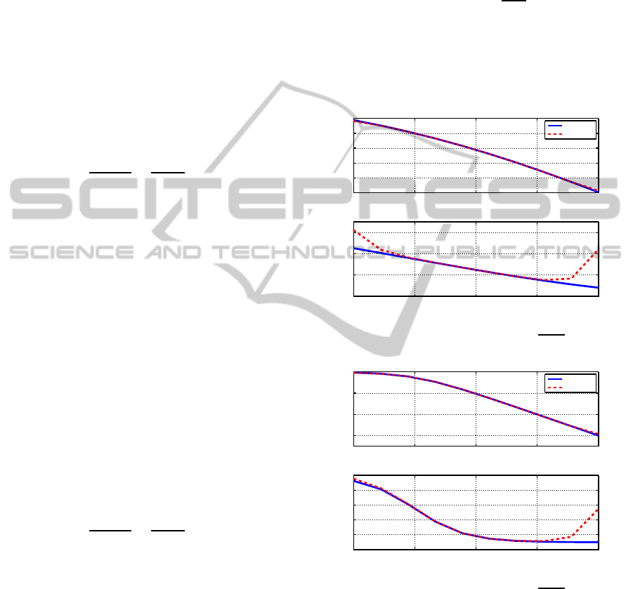
3.3.2 Frequency response of
1
s
α
+1
Figures below show the frequency domain validation
of the IO approximations for different values of α
(plot for α = 0.3 is not shown due to space con-
straints).
10
−2
10
0
10
2
10
4
10
6
−14
−12
−10
−8
−6
−4
Frequency in rad/s
Magnitude in decibels
FOTF
Oustaloup
10
−2
10
0
10
2
10
4
10
6
−8
−6
−4
−2
Frequency in rad/s
Phase in degrees
Figure 1: Bode Plot for G
1
(s) =
1
s
0.1
+1
.
10
−2
10
0
10
2
10
4
10
6
−60
−40
−20
0
Frequency in rad/s
Magnitude in decibels
FOTF
Oustaloup
10
−2
10
0
10
2
10
4
10
6
−50
−40
−30
−20
−10
0
Frequency in rad/s
Phase in degrees
Figure 2: Bode Plot for G
3
(s) =
1
s
0.5
+1
.
It can be observed that for the frequency range of 10
0
to 10
4
rad/sec we get an exact match for the frequency
response, which advocates that the obtained approxi-
mation can replace the original FOTF for the said fre-
quency range.
SIMULTECH2014-4thInternationalConferenceonSimulationandModelingMethodologies,Technologiesand
Applications
364

10
−2
10
0
10
2
10
4
10
6
−100
−80
−60
−40
−20
0
Frequency in rad/s
Magnitude in decibels
FOTF
Oustaloup
10
−2
10
0
10
2
10
4
10
6
−60
−40
−20
0
Frequency in rad/s
Phase in degrees
Figure 3: Bode Plot for G
4
(s) =
1
s
0.7
+1
.
10
−2
10
0
10
2
10
4
10
6
−120
−100
−80
−60
−40
−20
0
Frequency in rad/s
Magnitude in decibels
FOTF
Oustaloup
10
−2
10
0
10
2
10
4
10
6
−100
−80
−60
−40
−20
0
Frequency in rad/s
Phase in degrees
Figure 4: Bode Plot for G
5
(s) =
1
s
0.9
+1
.
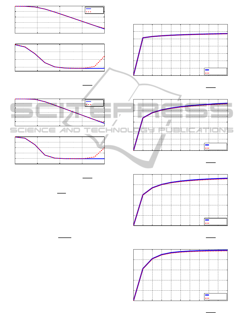
3.3.3 Step Response of
1
s
α
+1
To obtain the expression for step response of FO
plant, the transfer function (9) is rewritten such that
an expression can be obtained in terms of Y(s) and
U(s), where the first is output and the later is the in-
put.
Y(s) =
U(s)
s
α
+ 1
. (16)
Now for step input U(s) = 1/s and then applying
inverse Laplace transformation (Monje et al., 2010),
gives:
Y(t) = 1− E
α
(−t
α
), (17)
where E
α
(−t
α
) is one parameter Mittag-Leffler Func-
tion (MLF) (Podlubny et al., 2002). Figures below
show the time domain validation of the IO approxi-
mations for different values of α (plot for α = 0.3 is
not shown due to space constraints).
From both frequency and step response it is ob-
served that the dynamics of original FO system is still
retained in the obtained IO approximation and hence
using this approximation for analysis and simulation
in model predictive control as a finite-dimensional
model of original FO system is justified.
0 1 2 3 4 5 6 7 8 9 10
0
0.1
0.2
0.3
0.4
0.5
0.6
0.7
Time in seconds
Output in units
FO
Approximation
Figure 5: Step response of G
1
(s) =
1
s
0.1
+1
.
0 1 2 3 4 5 6 7 8 9 10
0
0.1
0.2
0.3
0.4
0.5
0.6
0.7
0.8
0.9
Time in seconds
Output in units
FO
Approximation
Figure 6: Step response of G
3
(s) =
1
s
0.5
+1
.
0 1 2 3 4 5 6 7 8 9 10
0
0.2
0.4
0.6
0.8
1
Time in seconds
Output in units
FO
Approximation
Figure 7: Step response of G
4
(s) =
1
s
0.7
+1
.
0 1 2 3 4 5 6 7 8 9 10
0
0.2
0.4
0.6
0.8
1
Time in seconds
Output in units
FO
Approximation
Figure 8: Step response of G
5
(s) =
1
s
0.9
+1
.
ModelPredictiveControlforFractional-orderSystem-AModelingandApproximationBasedAnalysis
365

4 MODEL PREDICTIVE
CONTROL
In this section, the theory of MPC is discussed in de-
tail.
4.1 Principle of Model Predictive
Control
For a system, the reference trajectory r(k) is defined as
the ideal trajectory along which a plant should return
to the set-point trajectory w(k), at any instant k. The
current error between the output signal y(k) and the
setpoint is an error represented as:
err(k) = w(k) − y(k). (18)
Then the reference trajectory is chosen such that if the
output followed it exactly, then the error after i steps
would be
err(k + i) = exp
−iT
s
/T
ref
err(k), (19)
where T
ref
is the time constant of exponential assum-
ing that reference trajectory approaches the set-point
exponentially and T
s
is the sampling interval. There-
fore, the reference trajectory is defined as
r(k + i|k) = w(k+ i) − y(k + i). (20)
The notation r(k + i|k) implies that the reference
trajectory depends on the conditions at time k
(J.M.Maciejowski, ) (Boudjehem and Boudjehem,
2012).
Now, the predictive controller uses an internal
model to estimate the future behavior of the plant.
This process starts at the current time k and carries
over a future prediction horizon H
P
. This predicted
behavior depends on the assumed control effort tra-
jectory ˆu that is to be applied over the prediction hori-
zon and we have to select the input which promises
the best predicted behavior. The notation ˆu represents
the predicted value input at time k + i at instant k; the
actual input u(k + i) may be different than ˆu. After a
future trajectory is decided, only the first element of
the trajectory is required as the control input to the
process. Hence u(k) becomes ˆu(k|k). The tasks of
prediction, measurement of output and determination
of input trajectory are repeated at every sampling in-
stant. This is known as the receding horizon strategy,
since prediction horizon slides along by one sampling
interval at each step while its length remains the same.
Formulation of MPC problem needs few basic el-
ements such as model, cost function, prediction equa-
tions and control law. These are covered in the next
section.
4.2 Problem Formulation
In MPC, the first element of paramount importance is
the model of the process/plant, which is required for
prediction of the future states. This model must show
the dependance of the output on the current measured
variable and the current inputs. A precise model will
deliver accurate predictions, but for MPC we do not
always need precise model though they are always
appreciated. Since the decisions that is, the optimal
control effort is updated regularly, any model uncer-
tainty can be dealt within a fair range (Rossiter, 2003).
Hence, accuracy of the model used for the prediction
can be compensated with regular updating of states.
In this paper, FO system is used as a plant/process.
Transfer function of the FO plant is:
G(s) =
1
s
α
+ 1
, (21)
where α is varied between 0 and 1.
Second element is the cost function, which is re-
quired to evaluate the input trajectory such that it
minimizes/maximizes the cost function. Selection of
the cost function is a crucial issue and involves engi-
neering and theocratical expertise. The cost function
should be as simple as one can get away with for the
desired performance. Choice of cost function affects
the complexity of the implied optimization and hence
it should taken into consideration that the cost func-
tion should be simple enough to have a straightfor-
ward optimization (Rossiter, 2003). For this reason 2-
norm measures are popular and the cost function used
in this paper is also a 2-norm measure.
J =
n
y
∑
i=1
kr
k+i
− y
k+i
k
2
2
+ λ
n
u
−1
∑
i=0
k∆u
k+i
k
2
2
(22a)
=
n
y
∑
i=1
ke
k+i
k
2
2
+ λ
n
u
−1
∑
i=0
k∆u
k+i
k
2
2
, (22b)
where λ is the weighting scalar; first term represents
the sum of squares of the predicted tracking errors
from an initial horizon to an output horizon n
y
and
the second term represents the sum of squares of the
control over the control horizon n
u
. It is assumed that
control increments are zero beyond the control hori-
zon, that is
∆u
k+i|k
= 0,i ≥ n
u
.
The third element is the optimization, which is used to
evaluate the control law. The control law is computed
from the minimization of the cost J (22a) with respect
to n
u
future control moves, that is ∆ u
−→
. It is denoted
SIMULTECH2014-4thInternationalConferenceonSimulationandModelingMethodologies,Technologiesand
Applications
366

as
J
min
∆ u
−→
= k r
−→
− y
−→
k
2
2
+ λk∆ u
−→
k
2
2
, (23a)
= k e
−→
k
2
2
+ λk∆ u
−→
k
2
2
, (23b)
where
r
−→
=

r(k + 1) r(k + 2) ···

T
. (24)
y
−→
=

y(k+ 1) y(k+ 2) ···

T
. (25)
∆u
−→
=

u(k+ 1) u(k+ 2) ···

T
. (26)
Once the model and the cost function is defined, next
step is to get prediction equations and these are ob-
tained from discrete state-space model of the plant.
4.3 Prediction with State-space Models
Prediction with a state-space model is straightfor-
ward, provided the nature of the model should be
strictly proper. Proof for prediction equation is as fol-
lows: Consider the state-space model which gives the
one step ahead prediction:
x
k+1
= Ax
k
+ Bu
k
; y
k+1
= Cx
k+1
, (27a)
and at instant k+ 2
x
k+2
= Ax
k+1
+ Bu
k+1
; y
k+2
= Cx
k+2
. (27b)
Substitute (22a) into (22b) to eliminate x
k+1
, we get
x
k+2
= A
2
x
k
+ ABu
k
+ Bu
k+1
; y
k+2
= Cx
k+2
, (27c)
at instant k+ 3 using (22c)
x
k+3
= A
2
x
k+1
+ ABu
k+1
+ Bu
k+2
; y
k+3
= Cx
k+3
. (27d)
Substitute (22a) to eliminate x
k+1
x
k+3
= A
2
[Ax
k
+ Bu
k
] + ABu
k+1
+ Bu
k+2
; y
k+3
= Cx
k+3
.
(27e)
Hence a generalized equation for n-step ahead predic-
tions will be
x
k+n
= A
n
x
k
+ A
n−1
Bu
k
+ A
n−2
Bu
k+1
+ . . . + Bu
k+n−1
,
(27f)
y
k+n
= C[A
n
x
k
+ A
n−1
Bu
k
+ A
n−2
Bu
k+1
+ . . . + Bu
k+n−1
].
(27g)
Hence, one can form the whole vector of future
predictions up to a horizon n
y
as follows:






x
k+1
x
k+2
x
k+3
.
.
.
x
k+n
y






=







A
A
2
A
3
.
.
.
A
n
y







x
k
+ H
x






u
k
u
k+1
u
k+2
.
.
.
u
k+n
y
−1






,
(28a)






y
k+1
y
k+2
y
k+3
.
.
.
y
k+n
y






=







CA
CA
2
CA
3
.
.
.
CA
n
y







x
k
+ H






u
k
u
k+1
u
k+2
.
.
.
u
k+n
y
−1






,
(28b)
H
x
=







B 0 0 ...
AB B 0 ...
A
2
B AB B ...
.
.
.
.
.
.
.
.
.
.
.
.
A
n
y
−1
B A
n
y
−2
B A
n
y
−3
B ...







,
(28c)
H =







CB 0 0 ...
CAB CB 0 ...
CA
2
B CAB CB .. .
.
.
.
.
.
.
.
.
.
.
.
.
CA
n
y
−1
B CA
n
y
−2
B CA
n
y
−3
B ...







.
(28d)
4.4 Discrete State-space Model for FO
Plants
In this paper, discrete state-space model is used in
MPC for tracking problem. Discrete state-space
model is obtained using Oustaloup recursive approx-
imation. As discussed in the above section, the state-
space model considered for prediction equations was
of strictly proper nature. However, the state-space
model obtained for five FO systems were not of
strictly proper nature and hence, a pole was added at
a far-away location in the left half of s-plane to make
the system strictly proper in nature. A state-space
model thus obtained was verified using frequency and
step response (refer subsection 3.3) and it was ob-
served that the addition of pole affects the frequency
response at higher frequencies. Thus, for a specific
region of frequency plot (from 10
0
to 10
4
rad/sec) the
FO system retains its original form. Finally, obtained
state-space model were discretized at a step size of 1
second. One example of discrete state-space model
obtained using approximation method is shown sub-
sequently.
ModelPredictiveControlforFractional-orderSystem-AModelingandApproximationBasedAnalysis
367

4.4.1 Discrete State-space Model for
1
s
0.5
+1
Expression (14) was used to obtain the discrete state-
space model (using MATLAB) with step size of one
second. The obtained A,B,C and D matrices are as
follows:
A =

A1 −6.934e
34
I 0

,
where, I is 10X10 identity matrix and A1 is single
row of 10 elements given by:
A1 = [−6.31e
15
,−1.886e
21
,−7.732e
25
,−4.944e
29
,
−5.064e
32
,−8.492e
34
,−2.426e
36
,−1.258e
37
,
−1.253e
37
,−2.354e
36
],
B = [1, 0, 0, 0, 0, 0, 0, 0, 0, 0, 0]
T
,
C = [6.303e
12
,4.726e
18
,4.848e
23
,7.714e
27
,1.939e
31
,
7.72e
33
,4.87e
35
,4.867e
36
,7.683e
36
,1.882e
36
,6.303
e
34],
D = 0.
Similarly, discrete state-space models for other
four FO plants were obtained. Once again the fre-
quency and step response of obtained state-space
model were compared with that of the original FOTF
and it was observed that conversion of transfer func-
tion to state-space does not affect frequency and step
response. Hence, use of state-space model (obtained
through approximation) instead of FO system is fur-
ther justified.
Once the model, cost function and the prediction
equations are defined for MPC; the next step is to
evaluate the control law.
4.5 Control Law
As stated above, the control law is determined from
the minimization of a 2-norm measure of predicted
performance (23). True optimal control uses n
y
=
n
u
= ∞ in performance index (Rossiter, 2003); but
there is a limitation on MPC algorithms and hence this
assumption cannot be validated, making MPC subop-
timal. Though an upper limit on n
y
and n
u
cannot be ∞
but the limits should be selected such that they are al-
ways higher than the settling time of the system. For
large n
y
and n
u
MPC gives near identical control to
an optimal control law with the same weights. While
on the other hand, very small n
y
and n
u
will result in
severely suboptimal control law (Rossiter, 2003)(Ca-
macho and Bordons, 2004). Hence, proper choice of
n
y
and n
u
is required for MPC. Selection of n
y
and n
u
will affect the control law, since they are calculated
ones and used each time when the control law is up-
dated. The control law for discrete state-space model
and unconstrained condition is (Rossiter, 2003):
∆u
k
= P
r
r
−→
− Kx− P
r
[y
k
− ˆy
k
], (30)
where y
k
is the process output (real output) and ˆy
k
is
the model output. P
r
and K are given by
P
r
= (H
T
H + λI)
−1
H
T
M,
K = (H
T
H + λI)
−1
H
T
P,
P =







CA
CA
2
CA
3
.
.
.
CA
n
y







,
and M is a weighting vector.
Expression (30) is used to evaluate optimal con-
trol effort u
∗
to be given to the plant/process and to
the model. At each instant the optimal control effort
u
∗
is updated by evaluating the control law (30) by
considering revised process output y
k
, model output
ˆy
k
and the states x. Fig. (9) represents block diagram
of MPC with FO plant and a model, obtained using
approximation method.
Optimizer
FO Plant
Model
X
y
k
ˆy
k
Ref
(r)
online
states
x
m
computation
+
−
u
∗
Figure 9: Block Diagram for MPC.
4.6 Process Output Evaluation
When MPC is applied to a real process, its output y
k
is
measured in real time at everyinstant for evaluation of
optimal control effort. In case of simulations, gener-
ally the model of the process/plant is used to evaluate
the process output. Hence, the bias [y
k
− ˆy
k
] is redun-
dant as y
k
is equal to ˆy
k
at each instant. In this paper,
the process output y
k
has been evaluated by formu-
lating an output equation in time domain for the input
given at each instant to the FO plant mentioned in (21)
for respective α values. Expression of y
k
in time do-
main was obtained by applying inverse Laplace trans-
formation ((Monje et al., 2010)) to the expression ob-
tained using transfer function of FO plant (9) for re-
spective α values. Laplace transform of Caputo frac-
tional differentiation (1) and a special function known
SIMULTECH2014-4thInternationalConferenceonSimulationandModelingMethodologies,Technologiesand
Applications
368

as Mittag-Leffler function (MLF) is used to evalu-
ate the expression of process output in time domain.
For the evaluation of process output expression, def-
initions of 1-parameter MLF, 2-parameter MLF and
Laplace transform of Caputo derivative is required
and they are as follows:
Definition for Laplace transform of Caputo fractional
differentiation is (Podlubny et al., 1997)
L[
C
0
D
α
t
f(t)] = s
α
F(s) −
m−1
∑
k=0
s
α−k−1
[
d
k
dt
k
f(t)]
t=0
,
(31)
where 0 < α < 1, m− 1 < α ≤ m and m ∈ N.
Definition for 1-parameter MLF is (Podlubny et al.,
2002)
E
α
=
∞
∑
k=0
t
k
Γ(αk+ 1)
, (32)
where α ∈ R
+
.
Definition for 2-parameter MLF is (Podlubny et al.,
2002)
E
α,β
=
∞
∑
k=0
t
k
Γ(αk+ β)
, (33)
where α,β ∈ R
+
.
Analytical expression for process output y
k
is ob-
tained by using inverse Laplace transformation on the
expression by rewriting transfer function (9) in terms
of Y(s) andU(s) using definition of Caputo fractional
differentiation (1) and using Laplace transform of Ca-
puto fractional differentiation (31) as follows:
Y(s)
U(s)
=
b
s
α
+ a
. (34a)
Above expression is a general form of (9)
s
α
Y(s) + aY(s) = bU(s). (34b)
The actual FDE with Caputo differentiation is
C
0
D
α
t
y(t) + ay(t) = bu(t), (34c)
for 0 < α < 1. Taking Laplace transform as given in
(31) for Caputo differentiation, we get
s
α
Y(s) −Y(0) + aY(s) = bU(s), (34d)
Y(s) =
bU(s)
s
α
+ a
+
Y(0)
s
α
+ a
. (34e)
Taking inverse Laplace transform we get
L
−1

bU(s)
s
α
+ a

= L
−1

1
s
α
+ a

∗ L
−1
(bU(s)).
(34f)
Note that u(t) is a constant value at any k
th
instant and
hence U(s) =
u
k−1
s
whereas u
k−1
is the constant value
obtained as the optimal control effort at the previous
instant. Using the standard inverse Laplace transform
expressions as given in (Monje et al., 2010), (34f) be-
comes
L
−1

bU(s)
s
α
+ a

= b× u
k−1
[1− E
α
(−at
α
)]. (34g)
Again using (Monje et al., 2010) for Laplace inverse
of second term
L
−1

Y(0)
s
α
+ a

= y(o) × [(t
α−1
)E
α,α
(−at
α
)]. (34h)
Hence, y
k
is obtained for using (34g) and (34h) as:
y
k
= b×u
k−1
[1−E
α,1
(−at
α
k
)]+y
k−1
[t
α−1
k
E
α,α
(−at
α
k
)].
(35)
Now, by substituting a = 1 and b = 1 in (35), an
expression for y
k
can be obtained for FO plant de-
scribed by (9) and this expression takes into account
intial/current conditions of plant.
y
k
= u
k−1
[1− E
α,1
(−t
α
k
)] + y
k−1
[t
α−1
k
E
α,α
(−t
α
k
)]
(36)
In the following section, results obtained for simula-
tion of unconstrained MPC with FO plant with differ-
ent α values are shown, where (0 < α < 1).
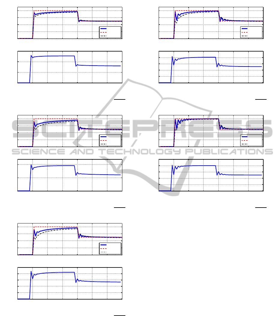
5 RESULTS
In the previous sections of this paper, the control law
and the process output has been evaluated which were
used to obtain these results. MPC is applied to an
FO plant defined at (21) for five different values of
α = 0.1,0.3, 0.5,0, 7 and 0.9. Simulations are car-
ried out to obtain output and input values for uncon-
strained condition. Output plot shows reference, pro-
cess output y
k
and model output ˆy
k
for respective FO
plants. Subsequent plot shows the optimal control ef-
fort u
∗
at each instant for respective plants. For all
plots y-axis represents amplitude in units and x-axis
represents sampling instances. Sampling time of 1
second is used for these results. Though here results
of simulations for one sampling time are shown, it
was observed that the simulation of MPC for these
FO plants is also possible for other step sizes. The
range of step size for which simulations can be car-
ried out was found to be from 0.5 to 1 seconds. This
becomes one of the advantages of using continuous
approximation methods for MPC of FO systems.
ModelPredictiveControlforFractional-orderSystem-AModelingandApproximationBasedAnalysis
369

0 10 20 30 40 50 60 70
0
0.2
0.4
0.6
0.8
Output plot
Process
Reference
Model
0 10 20 30 40 50 60 70
0
0.5
1
1.5
Control Effort
Figure 10: Output and control effort for G
1
(s) =
1
s
0.1
+1
.
0 10 20 30 40 50 60 70
0
0.2
0.4
0.6
0.8
Output plot
Process
Reference
Model
0 10 20 30 40 50 60 70
0
0.5
1
Control Effort
Figure 11: Output and control effort for G
2
(s) =
1
s
0.3
+1
.
0 10 20 30 40 50 60 70
0
0.2
0.4
0.6
0.8
Output plot
Process
Reference
Model
0 10 20 30 40 50 60 70
0
0.2
0.4
0.6
0.8
1
Control Effort
Figure 12: Output and control effort for G
3
(s) =
1
s
0.5
+1
.
Process output and model output are seen to have dif-
ferent values initially because both are calculated us-
ing different equations, though same initial conditions
are fed to both the models . Process output is calcu-
lated using (36) with the help of MATLAB routine
mlf() developed by Podlubny. Model output is cal-
0 10 20 30 40 50 60 70
0
0.2
0.4
0.6
0.8
Output plot
Process
Reference
Model
0 10 20 30 40 50 60 70
0
0.2
0.4
0.6
0.8
1
Control Effort
Figure 13: Output and control effort for G
4
(s) =
1
s
0.7
+1
.
0 10 20 30 40 50 60 70
0
0.2
0.4
0.6
0.8
Output plot
Process
Reference
Model
0 10 20 30 40 50 60 70
0
0.2
0.4
0.6
0.8
1
Control Effort
Figure 14: Output and control effort for G
5
(s) =
1
s
0.9
+1
.
culated using state-space model using (27) obtained
through Oustaloup recursive approximation. It was
observed that the difference between process output
and model output eventually becomes negligible. Re-
sults clearly show that the optimal control effort is ob-
tained so that the process output can track the refer-
ence signal. In real scenario, there will be a actual
plant running and on that MPC will be applied. It
will be possible to measure real output at every in-
stant and that will be fed to the optimizer along with
the calculated output of internal model (see Fig. (9)).
In most of the cases there will be a small amount of
difference in the actual output and the model output
at initial stages due to the errors in the model of the
process. Here in simulations, the same scenario was
created by using process output expression instead of
using the same state-space model which was used as
an internal model.
Few observations are noted from these results.
Magnitude of control effort goes on reducing as the
fractional-order α goes on increasing. Also, the pro-
cess output becomes more oscillatory with increasing
SIMULTECH2014-4thInternationalConferenceonSimulationandModelingMethodologies,Technologiesand
Applications
370

α value, when the reference signal changes. There are
two different reasons which may cause these anoma-
lies. As stated earlier, control effort is obtained so that
the process output can track the reference signal and
hence process output expression is the reason behind
this reduction. Process output expression uses two
MLFs for its computation (see (36), (32) and (33)).
MLF takes a long time for computation and the na-
ture of MLF changes very rapidly for small α values.
The other reasons behind irregularity can be the infi-
nite memory nature of the FO system. For small α
values a larger amount of past values are considered
for computation.
Both these observations are not seen as soon as
constraints are applied on the input as well as out-
put. In this paper, unconstrained case was considered
since for an optimal solution one needs to first con-
firm that solution exists for unconstrained case before
going to constrained situation. In optimal theory, it is
said that if the control law does not deliveroptimal so-
lution and robustness in the unconstrained case then it
will not give optimal solution in the constrained case
(Rossiter, 2003). Unfortunately the opposite does not
hold true and hence it is worthwhile to check the per-
formance of the system for unconstrained case first.
From these results it is evident that FO system’s
model can be used in its true form using approxima-
tion method for MPC. Furthermore, the obtained pro-
cess and model output depicts the behaviour of the
original FO system in terms of nature of plot and the
required settling time. Systems with small values of α
tend to take large time to settle. The reference trajec-
tory is followed faithfully. The reference signal used
for the simulation contains both positive and negative
steps and hence it can be inferred that MPC for FO
systems can work for all types of limiting reference
signals.
6 CONCLUSION
Fractional-order systems are represented using FO
model and for MPC, the model is required for pre-
diction purposes. A discrete state-space model de-
livers straightforward prediction equations with one
condition that the model should be of strictly proper
nature. Control law was obtained for unconstrained
MPC problem and was utilized to obtain results.
It was observed that MPC can be utilized for FO
plants once the model of the FO plant is obtained and
a unique analytical expression can be used to depict
process output for FO plants. Approximation method
was used to obtain model of the FO plant and its au-
thenticity was verified using frequency and step re-
sponse. Obtained results reveal that MPC can be used
for FO plants and the model used works fine. More-
over, use of systematic expression obtained for pro-
cess output makes it realistic. Hence, classical servo
problem can be solved for a class of linear FO systems
with the help of approximation method using MPC.
Use of other approximation methods like modi-
fied Oustaloup, Carlson will be interesting for MPC
of FO systems. Furthermore, a comparison of these
approximation methods for a single FO system might
reveal some motivating results and hence the study of
MPC with constraints for FO systems would be quite
interesting and worth exploring as a future scope.
REFERENCES
Bemporad, A. (2006). Model predictive control design:
New trends and tools. IEEE Conference on Decision
and Control.
Boudjehem, D. and Boudjehem, B. (2012). A fractional
model predictive control for fractional order systems.
Fractional Dynamics and Control Springer, pages 59–
71.
Camacho, E. and Bordons, C. (2004). Model Predictive
control, volume 2. Springer.
Caponetto, R., Dongola, G., and Fortuna, L. Fractional Or-
der Systems Modeling and Control Applications, vol-
ume 72. World Scientific Publishing Co. Pvt. Ltd.,
second edition.
Dzieli´nski, A. and Sierociuk, D. (2010). Fractional or-
der model of beam heating process and its experi-
mental verification. In New trends in nanotechnology
and fractional calculus applications, pages 287–294.
Springer.
Enacheanu, O., Riu, D., Reti`ere, N., Enciu, P., et al. (2006).
Identification of fractional order models for electrical
networks. In Proceedings of IEEE Industrial Elec-
tronics IECON 2006–32nd Annual Conference on,
pages 5392–5396.
Gabano, J.-D. and Poinot, T. (2011). Fractional modelling
and identification of thermal systems. Signal Process-
ing, 91(3):531–541.
Garcia, C., Prett, D., and Morari, M. (1989). Model predic-
tive control: Theory and practice-a survey. Automat-
ica, 25(3):335–348.
Hortelano, M. R., de Madrid y Pablo, A. P., Hierro, C., and
Berlinches, R. H. (2010). Generalized predictive con-
trol of arbitrary real order. New trends in nanotechnol-
ogy and fractional calculus applications, Springer.
J.M.Maciejowski. Predictive Control with Constraints.
Prentice Hall.
Mansouri, R., Bettayeb, M., and Djennoune, S. (2010). Ap-
proximation of high order integer systems by frac-
tional order reduced-parameters models. Mathemat-
ical and Computer Modelling, 51(1):53–62.
ModelPredictiveControlforFractional-orderSystem-AModelingandApproximationBasedAnalysis
371

Monje, C. A., Chen, Y. Q., Vinagre, B. M., Xue, D., and Fe-
liu, V. (2010). Fractional Order Systems and Control.
Springer.
Morari, M. and Lee, J. H. (1999). Model predictive control:
past, present and future. The Journal of Computers
and Chemical Engineering.
Muske, K. R. and Rawlings, J. B. (1993). Model predictive
control with linear models. Process Systems Engineer-
ing, 39(2):262–287.
Nise, N. S. (2007). Control Systems Engineering. John
Wiley & Sons.
Podlubny, I. (1998). Fractional differential equations: an
introduction to fractional derivatives, fractional dif-
ferential equations, to methods of their solution and
some of their applications, volume 198. Academic
press.
Podlubny, I., Dorcak, L., and Kostial, I. (1997). On frac-
tional derivatives, fractional-order dynamic systems
and pi
λ
d
µ
-controllers. volume 5, pages 4985–4990.
36th IEEE Conference on Decision and Control.
Podlubny, I., Petras, I., Vinagre, B. M., O’leary, P., and Dor-
cak, L. (2002). Analogue realizations of fractional-
order controllers. J.Nonlinear Dynamics, 29.
Poinot, T. and Trigeassou, J.-C. (2003). A method for mod-
elling and simulation of fractional systems. Signal
processing, 83(11):2319–2333.
Poinot, T. and Trigeassou, J.-C. (2004). Identification of
fractional systems using an output-error technique.
Nonlinear Dynamics, 38(1-4):133–154.
Rawlings, J. B. (2000). Tutorial overview of model predic-
tive control. IEEE Control Systems Magazine.
Romero, M., de Madrid, A. P., Maoso, C., and Vinagre,
B. M. (2010). Fractional order generalized predictive
control: Formulation and some properties. Int. Conf.
Control, Automation, Robotics and Vision Singapore.
Rossiter, J. A. (2003). Model - Based Predictive Control: A
Practicle Approach. CRC Press.
Valerio, D. and Costa, J. (2011). Variable order fractional
order derivatives and their numerical approximations.
J. Signal Processing, 91.
Vinagre, B. M., Podlubny, I., Hernandez, A., and Feliu, V.
(2000). Some approximation of fractional order op-
erators used in control theory and applications. Frac-
tional calculus and applied analysis, 3(3):210–213.
YaLi, H. and Ruikun, G. (2010). Application of fractional
order model reference adaptive control on industry
boiler burning system. Int. Conf. on intelligent Com-
putation Technology and Automation.
SIMULTECH2014-4thInternationalConferenceonSimulationandModelingMethodologies,Technologiesand
Applications
372