A Pursuit-evasion Game Between Unmanned Aerial Vehicles

Alexander Alexopoulos, Tobias Schmidt and Essameddin Badreddin

Automation Laboratory, Institute for Computer Engineering, Heidelberg University, B6, Mannheim, Germany

Keywords:

Pursuit-evasion Games, Dynamic Non-cooperative Games, Unmanned Aerial Vehicles, Quad-rotors, Real-

time Applications.

Abstract:

In this paper the problem of two-player pursuit-evasion games with unmanned aerial vehicles (UAVs) in a

three-dimensional environment is solved. A game theoretic framework is presented, which enables the solution

of dynamic games in discrete time based on dynamic programming. The UAV agents taking part in the pursuit-

evasion game are two identical quad-rotors with the same non-linear state space model, while the evaders’

absolute velocity is smaller than the pursuers’. The convergence of the pursuit-evasion game is shown in

numerical simulations. Finally, the approach is simulated on an embedded computer and tested for real-time

applicability. Hence, the implementation and real-time execution on a physical UAV system is feasible.

1 INTRODUCTION

In recent years, pursuit-evasion games (PEGs) are

highly challenging problems in the research area of

optimal control theory and robotics. Generally, in

PEGs a pursuer (or a team) are supposed to cap-

ture an evader (or a team) that is trying to escape.

Many applications and areas of operations are con-

ceivable, e.g., search and rescue missions, cops and

robber games, patrolling, surveillance, and warfare.

In robotics, there exist two primary approaches for

solving PEGs: combinatorial and differential. The

former requires the environment being represented ei-

ther geometrically (e.g., with polygons) or topologi-

cally (e.g., by a graph). The Lion and Man problem

is a famous example of PEGs. According to (Nahin,

2012), it is deemed to be one of the ﬁrst (unpub-

lished) mathematically formulated PEGs, deﬁned by

R. Rado in the 1920s. The problem was extensively

studied, e.g., by Littlewood (Littlewood, 1986) and

Sgall (Sgall, 2001). The former tackles the problem

in continuous time and space, while, on the contrary,

the latter analyzes it in discrete time.

The authors of (Chung et al., 2011) summarized

different approaches for solving PEGs, which are ap-

plicable in robotics. They aimed to survey methods

that are based on combinatorial approaches.

Earlier, LaValle and Hutchinson surveyed

(LaValle and Hutchinson, 1993) various applications

in robotics, which are applicable for game theoretic

formulation. The focus of their survey is how

game theory can be applied to robot navigation,

high-level strategy planning, information gathering

through manipulation and/or sensor planning, and

pursuit-evasion scenarios.

Game-theoretic approaches consider that the so-

lution of a problem does not only depend on the own

decisions but on the decisions of each agent involved.

Those problems are solved assuming rational decision

making by all players. PEGs can be formulated as dy-

namic non-cooperative games, while the evolution of

the game state depends on the dynamic constraints of

each agent. Such dynamic PEGs (differential games)

where introduced by Isaacs (Isaacs, 1965), e.g., the

Homicidal Chauffeur Game. In this game a more ag-

ile but slower evader shall avoid to become run over

by a faster but curvature-bound pursuer. The agents

of such dynamic games are described by differential

equations, which characterize the agents’ dynamics.

The authors of (Vieira et al., 2009) published an

implementation of a PEG on mobile robots, where a

group of pursuers are supposed to catch a group of

evaders. They use game theory to solve the PEG. Un-

fortunately, the PEG is solved off-line and the cost of

the robots’ motions are stored as weights on a mathe-

matical graph. The motions of the robots are based on

the best path according to the edges’ weights between

the graphs’ vertices. This approach provides an open-

loop solution, because the agents cannot respond to

unpredictable events.

As far as is known, there is hardly anything

done in research area of PEGs with UAVs in three-

Alexopoulos A., Schmidt T. and Badreddin E..

A Pursuit-evasion Game Between Unmanned Aerial Vehicles.

DOI: 10.5220/0005038600740081

In Proceedings of the 11th International Conference on Informatics in Control, Automation and Robotics (ICINCO-2014), pages 74-81

ISBN: 978-989-758-040-6

 2014 SCITEPRESS (Science and Technology Publications, Lda.)

dimensional environment, thus, an implementation of

a PEG on real UAV systems seems not to be car-

ried out, yet. In this paper, a framework is pro-

posed, which provides a closed-loop solution of a

PEG with two UAVs based on game-theoretic meth-

ods in a three-dimensional environment. Since the so-

lutions (control actions of the UAVs) shall be calcu-

lated locally, the approachwas implemented on an on-

board embedded computer, running a real-time oper-

ating system (RTOS). This set-up assures that the pre-

deﬁned real-time speciﬁcations are satisﬁed. Hence,

the foundations for an implementation on a real UAV

system are laid.

In the next section the problem formulation is

stated and the corresponding solution approach is pre-

sented. In section 3, a brief system description of the

controlled UAV model is given. Section 4 introduces

the framework with which N-player discrete-time de-

terministic dynamic games can be solved. Then, the

two-player UAV PEG formulation is given in section

5. After that, the implementation of the PEG on the

embedded computer is described in section 6. Finally,

the simulation results and some interesting aspects

and remarks are discussed in sections 7 and 8.

2 PROBLEM STATEMENT AND

SOLUTION APPROACH

2.1 Problem Statement

Two UAV agents (pursuer and evader) with the same

dynamic constraints are given. The pursuer is able

to move faster through the three-dimensional environ-

ment than the evader. Furthermore, both UAVs have

an attitude and velocity controller implemented. The

agents are in a conﬂict situation called PEG. PEGs de-

scribe a problem, in which an agent tries to catch an

adversarial agent, while the meaning of catch is the

fulﬁlment of one or more conditions.

A solution to this game is sought that fulﬁls the

following requirements:

• Considering that the solution depends on deci-

sions of the antagonist, while each agent is aware

of that.

• Being able to react to unexpected behavior of the

adversarial agent (closed-loop solution).

• Computational time has to satisfy the determined

real-time speciﬁcations.

2.2 Solution Approach

Therefore, the following points were processed:

• Game-theoretical problem formulation as two-

player discrete-time deterministic dynamic zero-

sum game.

• Consideration of feedback (perfect state) infor-

mation structure and on-line computation of opti-

mal strategies by calculating the closed-loop Nash

equilibrium in mixed strategies in each discrete

time step.

• Implementation of the approach on an embedded

computer with RTOS.

3 SYSTEM DESCRIPTION

3.1 Dynamical Model

For modeling the quad-rotor dynamics, the mechan-

ical conﬁguration depicted in Figure 1 was assumed.

The body ﬁxed frame and the inertial frame are de-

noted by e

and e

, respectively. The UAV is deﬁned

as a point mass. To derive the equations of motions,

the following notations are necessary. P

= (x, y, z)

is the position vector of the quad-rotors’ center of

gravity in the inertial frame, P

= (x

, y

, z

)

is the

position vector of the quad-rotors’ center of gravity in

the body ﬁxed frame, v = (u, v, w)

are the linear ve-

locities in the body ﬁxed frame, ω = (p, q, r)

are the

angular rates for roll, pitch and yaw in the body ﬁxed

frame and Θ = (φ, θ, ψ)

is the vector of the Euler

angles. A key component of the quad-rotor model is

the transformation between inertial and body frames.

Rigid body dynamics are derived with respect to the

body frame that is ﬁxed in the center of gravity of the

quad-rotor. However, to simulate the motion of the

quad-rotor in the inertial frame, a transformation of

the coordinates is needed. If the quad-rotors’ attitude

is parameterized in terms of Euler angles, the trans-

formation can be performed using the rotation matrix

R(Θ), which is a function of roll, pitch and yaw an-

gles. Using s and c as abbreviations for sin(·) and

θ:Pitch

:Roll

:Yaw

Figure 1: Mechanical conﬁguration of a quadrocopter with

body ﬁxed and inertial frame.

APursuit-evasionGameBetweenUnmannedAerialVehicles

cos(·), respectively, the linear velocities deﬁned in the

inertial frame can be obtained as follows:

cθcψ sφsθcψ−cφsψ cφsθcψ+ sφsψ

cθsψ sφsθsψ− cφcψ cφsθsψ − sφcψ

−sθ sφcθ cφcθ

. (1)

The transformation of positions deﬁned in the body

frame into the corresponding positions in the inertial

frame can be obtained by







R(Θ) P

B,org

0 1





. (2)

The equations of motion are derived from the

ﬁrst principles (Newton-Euler laws (Beatty, 2006))

to describe both the translational and rotational

motion of the quad-rotor, leading to the follow-

ing discrete-time non-linear state space model with

the state vector x = [

]

[

]

, while s and c are abbre-

viations for sin(·) and cos(·), respectively:







k+1

























−(cx

+ sx

)

−(cx

+ sx

)

g− cx

− I

−

g(υ)

− I

−

g(υ)

− I







∆t, (3)

with υ = (υ

, υ

)

, υ ∈ ϒ being the inputs for

altitude, roll, pitch and yaw, I

, I

are the inertia

around x, y, z-axes, I

is the rotor moment of inertia,

L is the length between the center of gravity of the

UAV and the center of one rotor, g is the gravitation

constant, g(υ) is a function of υ depending on the ro-

tors’ angular velocities and ∆t is the sampling time.

The derivation of the model cannot be handled here

in detail. For more details on quad-rotor modeling

(Bouabdallah and Siegwart, 2007) can be consulted.

A closer look at the state space model reveals that the

angular accelerationsdepend only on the angular rates

and the input vector υ and the linear accelerations de-

pend on the Euler angles and υ. Hence, the state space

model can be divided into two interlinked sub-models

M1 and M2. Table 1 lists the chosen parameters based

on (Voos, 2009). In this paper, all values without unit

are normalized to the SI units.

Table 1: Model parameters.

Parameter Value

m 0.5

L 0.2

= I

4.85·10

−3

8.81·10

−3

3.36·10

−5

thrust factor 2.92·10

−6

air drag factor 1.12· 10

−7

3.2 Attitude and Velocity Control

The model structure is suitable for a cascaded attitude

and velocity controller. The attitude controller, con-

trolling subsystem M1, is ordered in the (faster) inner

loop and the velocity controller, controlling M2 in the

(slower) outer loop. The control of attitude and veloc-

ity of quad-rotors are not part of this work; therefor,

refer to (Voos, 2009) and (Krstic et al., 1995) for more

details about the present controller. More than sufﬁ-

cient reference reaction with the given control struc-

ture were derived in simulations (Alexopoulos et al.,

2013).

4 GAME-THEORETICAL

SOLUTION APPROACH

Game theory is an approach for strategic decision-

making, considering that the solution depends on the

decision of other agents, while everybody is aware of

that. This makes the solution process very complex,

especially if the number of players rises. Since PEGs

are highly competitive games, only non-cooperative

games are considered in this paper. Non-cooperative

games treat a conﬂict situation where increasing the

pay-off of one player results in decreasing that of an-

other. The following deﬁnition describes the class of

games considered in this work.

4.1 N-player Discrete-time

Deterministic Dynamic Games

A N-player discrete-time deterministic dynamic game

with a non-ﬁxed terminal time can be deﬁned by the

octuplet {N, K, X,U, f, ι, Γ, L} with:

• A set of players N = {1, . . . , N}.

• A set K = {1, . . . , K} denoting the stage of the

game.

ICINCO2014-11thInternationalConferenceonInformaticsinControl,AutomationandRobotics

• An inﬁnite set X, being the state space with the

states x

∈ X, ∀ k ∈ K∪ {K + 1}.

• A set U

, with k ∈ K and i ∈ N being the action

space of player i in stage k, where the elements u

are all admissible actions of player i in stage k.

• A difference equation f

: X × U

× U

× ·· · ×

→ X, deﬁned for each k ∈ K, so that

k+1

= f

, u

, . . . , u

), k ∈ K (4)

with x

∈ X as the initial state, describing the evo-

lution of a decision process.

• A ﬁnite set ι

, deﬁned for each k ∈ K and i ∈ N,

is the information structure of each player, while

the collection of all players information structures

ι is the information structure of the game.

• A class Γ

of functions γ

: X → U

deﬁned for

each k ∈ K and i ∈ N are the strategies of each

player i in stage k. The class Γ

is the collection

of all such strategies and is the strategy space of

player i.

• A functional L

: (X ×U

×·· ·×U

)×(X ×U

··· × U

) × · ·· × (X × U

× ··· × U

) → ℜ de-

ﬁned for each i ∈ N and is called cost functional

of player i.

The game stops as soon as the terminal set Ξ ⊂

X × {1, 2, ...} is reached, meaning for a given N-

tuple of actions in stage k, k is the smallest integer

with (x

, k) ∈ Ξ. With this deﬁnition it is possible to

describe the dynamic game in normal form (matrix

form). Each ﬁxed initial state x

and each ﬁxed N-

tuple of admissible strategies {γ

∈ Γ

;i ∈ N} yield a

unique set of vectors {u

, γ

(ι

), x

k+1

;k ∈ K, i ∈ N},

due to the causality of the information structure and

the evolution of the states according to a difference

equation. Inserting this vector in L

(i ∈ N) yields

a unique N-tuple of numbers, reﬂecting the costs of

each player. This implicates the existence of the map-

ping J

: Γ

× ·· · × Γ

→ ℜ for all i ∈ N, being also

the cost functional of player i with i ∈ N. According

to that, the spaces (Γ

, . . . , Γ

) and the cost functional

, . . . , J

) built the normal-form description of the

dynamic game with a ﬁxed initial state x

Since this class of games can be described in nor-

mal form, all solution concepts for non-cooperative

games, e.g., found in (Bas¸ar and Olsder, 1999), can be

used directly. For solving the later termed PEG with

UAV agents, the solution concept of Nash equilibrium

in mixed strategies (Nash, 1950) was used. Due to the

fact that the PEG in this work is formulated as a two-

player zero-sum game (Thomas, 1984), the saddle-

point equilibrium in mixed strategies is sought, while

being equivalent to the Nash equilibrium in zero-sum

games.

4.2 Saddle-point Equilibrium

A tuple of action variables (u

∗

, u

∗

) ∈ U,U = U

×U

in a two-player game with cost functional L is in

saddle-point equilibrium, if

L(u

∗

, u

) ≤ L(u

∗

, u

∗

) ≤ L(u

, u

∗

), ∀(u

, u

) ∈ U. (5)

This means that the order of the maximization and

minimization done is irrelevant:

min

∈U

max

∈U

L(u

, u

) = max

∈U

min

∈U

L(u

, u

) = L(u

∗

, u

∗

) =: L

∗

(6)

Note that if a value exists (a saddle-point exists), it

is unique, meaning if another saddle-point (ˆu

, ˆu

)

exists, L(ˆu

, ˆu

) = L

∗

applies. Moreover (u

∗

, ˆu

)

and ( ˆu

, u

∗

) constitute also a saddle-point. This fea-

ture does not hold for Nash equilibria (non-zero-sum

games). If there is no value in a zero-sum game,

min

∈U

max

∈U

L(u

, u

) > max

∈U

min

∈U

L(u

, u

) (7)

holds. Hence, there is no saddle-point solution.

Therefore, we consider the saddle-point equilibrium

in mixed strategies with the following property:

Theorem 1 (Minimax-Theorem) Each ﬁnite two-

player zero-sum game has a saddle-point equilibrium

in mixed strategies (von Neumann and Morgenstern,

2007).

4.2.1 Saddle-point Solution in Mixed Strategies

If there is no saddle-point solution in pure strategies,

the strategy space is extended, thus, the players can

choose their strategies based on random events, lead-

ing to the so called mixed strategies. That means, a

mixed strategy for a player i is a probability distribu-

tion p

over the action space U

. This holds also for

general games having no Nash equilibrium. To get

a solution in mixed strategies, L

is replaced by its

expected value, according to the chosen mixed strate-

gies, denoted by J

, p

). A 2-tuple (p

∗

, p

∗

) is a

saddle-point equilibrium in mixed strategies of a two-

player game, if

J(p

∗

, p

) ≤ J(p

∗

, p

∗

) ≤ J(p

, p

∗

), ∀(p

, p

) ∈ P, P = P

× P

(8)

holds, with J(p

, p

) = E

[L(u

, u

)]. Thus, J

∗

J(p

∗

, p

∗

) is called the value of the zero-sum game in

mixed strategies.

4.3 Discrete-time Dynamic Zero-sum

Games

4.3.1 Information Structure

It is assumed that a feedback information structure is

available to all agents during the game ι

= {x

}, k ∈

K, i ∈ N.

APursuit-evasionGameBetweenUnmannedAerialVehicles

4.3.2 Stage-additive Cost Functional

The cost functional for the discrete-time dynamic

game is formulated as follows:

L(u

, . . . , u

) =

∑

k=1

k+1

, u

, . . . , u

, x

), (9)

with u

= (u

′

, . . . , u

′

)

′

. This cost functional for

player i is called “stage-additive” and implies the ex-

istence of a g

: X × X ×U

× · ·· × U

→ ℜ, k ∈ K.

4.3.3 Dynamic Programming for Discrete-time

Dynamic Zero-sum Games

Since a stage-additive cost functional and a feed-

back information structure is assumed, dynamic pro-

gramming and the Principle of Optimality (Bellman,

1957) can be applied. Hence, the set of strategies

{γ

k∗

);k ∈ K, i = 1, 2} is for a two-player discrete-

time dynamic zero-sum game a feedback-saddle-point

solution if, and only if a functionV(k, ·) : ℜ

→ ℜ, k ∈

K exists, thus the following recursion is satisﬁed:

(k, x) = min

∈U

max

∈U



(x, u

, u

), u

, u

, x





k+ 1, f

(x, u

, u

)

i

= max

∈U

min

∈U



(x, u

, u

), u

, u

, x





k+ 1, f

(x, u

, u

)

i

= g



(x, γ

k∗

(x), γ

k∗

(x)), γ

k∗

(x), γ

k∗

(x), x





k+ 1, f

(x, γ

k∗

(x), γ

k∗

(x))



;

V(K+1, x) = 0.

(10)

The value function is found by calculating the saddle-

point equilibria in mixed strategies recursively for

each stage of the game as described above.

5 PURSUIT-EVASION GAME

FORMULATION

The PEG between the two UAV systems is deﬁned

with following characteristics:

• A set of two players {e, p}.

• A set K = {1, . . . , K} with variable number of

stages K. K is the time p needs to capture e, i.e.,

to minimize the distance d

to player e (e reaches

the terminal set Ξ). Thus, K depends on the initial

states of e and p.

• The terminal set Ξ ⊂ X × Y × Z × {1, 2, . . . } is

the set of all elements ξ ∈ Ξ of a sphere around

the pursuers’ position (x

, y

, z

) with radius d

stage k.

• A set X = X ×Y × Z ×U ×V ×W ×Φ× Θ× Ψ×

P× Q× R being the state space.

• Two ﬁnite discrete action spaces U

= U

⊂

U × V × W. U

and U

are steady during each

stage k of the game. They are deﬁned as U



pu,1

+ i

pu,2

− u

pu,1

, u

pv,1

+ j

pv,2

− u

pv,1

pw,1

+ l

pw,2

− u

pw,1



, with i = 0, . . . , s;

j = 0, . . . , s; l = 0, . . . , s and U

= U

, while

(s + 1)

is the number of strategies available for

each player and [u

pu,1

, u

pu,2

] = [u

pv,1

, u

pv,2

] =

pw,1

, u

pw,2

] = [u

eu,1

, u

eu,2

] = [u

ev,1

, u

ev,2

] =

ew,1

, u

ew,2

] = [−1, 1] are the continuous action

spaces. u

and u

are elements of the sets U

and

, while u ∈ U

×U

• The state of the PEG between two UAVs in the

pursuers reference frame is deﬁned as

= x

− x



















− x

− y

− z

− u

− v

− w

− φ

− θ

− ψ

− p

− q

− r



















(11)

with the difference function x

k+1

= f



, h(w

)



deﬁned in equation 3, while w

= u

− u

and

h : U ×V ×W → ϒ provides an input vector υ =

(υ

, υ

)

. Note that this state space model

describes the evolution of the PEG state relative

to the pursuer p.

• A feedback perfect state information structure

= ι

= {x

}, ∀k ∈ K.

• The strategy spaces Γ

= U

und Γ

= U

• A cost functional

J(p

, p

) = E

∑

k=1

D( f



, h(w

)



, x

)

, (12)

with D(·) being a function describing the change

in distance between p and e in one stage k, playing

the control action (u

, u

• The value function

V(k, x

) = min

max

J(p

, p

). (13)

ICINCO2014-11thInternationalConferenceonInformaticsinControl,AutomationandRobotics

• p

k∗

= (p

k∗

, p

k∗

) is the optimal solution of the

game in stage k. It is calculated by solving

the closed-loop saddle-point equilibrium in mixed

strategies. The optimal probability distributions

k∗

= (p

k∗

, p

k∗

) over the action space U

×U

stage k is given by

k∗

= argV(k, x

), ∀k ∈ K. (14)

• The optimal control actions u

k∗

= (u

k∗

, u

k∗

) are

those where the probabilities p

k∗

and p

k∗

are max-

imal. The reference velocities for the pursuers’

and evaders’ velocity controller are given by

r,k

= (u

, v

, w

)

+ (u

k∗

)

(15)

and

r,k

= (u

, v

, w

)

+ (u

k∗

)

. (16)

Since the solution of the above described prob-

lem shall be computed in real-time, the embedded

computer and the implementation of the PEG are pre-

sented in the following section.

6 IMPLEMENTATION

The implementation of the pursuit-evasion problem

deﬁned above on an embedded computer is brieﬂy

described in this section. Firstly, the utilized em-

bedded computer is described. Then, an algorithm is

described, which enables the determination of Nash

equilibria in mixed strategies of N-player games. Fi-

nally, a pseudo code is given describing the overall

solution process of the PEG.

6.1 Embedded Computer

There are many low-power and small-size comput-

ers available, e.g., Raspberry Pi (Raspberry Pi Foun-

dation, 2014), Cubieboard (CubieTech Ltd., 2014),

BeagleBoard (Texas Instruments Inc., 2014a), and

some variants. Many of those single-board comput-

ers are open-source hardware, assembled with a low-

frequency processor. For this work a BeagleBone

Black (Texas Instruments Inc., 2014b) was utilized,

a community-supported development platform with a

TI Sitara AM335x 1GHz ARMCortex A8 processor

and 512MB DDR3 RAM. The embedded computer

runs with QNX 6.5, a RTOS enabling the implemen-

tation and execution of real-time applications written

in C programming language.

6.2 Algorithm for N-player

Nash-equilibrium in Mixed

Strategies

As described above, an optimal control action tuple

k∗

= (u

k∗

, u

k∗

) for the agents p and e in stage k of

the PEG is derived by the determination of the Nash

(saddle-point) equilibrium. The MATLAB-function

NPG (Chatterjee, 2010) is able to solve an N-player

ﬁnite non-cooperative game by computing one Nash

equilibrium in mixed strategies. Thereby, the opti-

mization formulation of a N-player non-cooperative

game according to (Chatterjee, 2009) is used for com-

putation. The function uses the sequential quadratic

programming based quasi Newton method to solve

a non-linear minimization problem with non-linear

constraints.

Since it is not feasible to generate C code of the

NPG function automatically, the algorithm to compute

one Nash equilibrium was implemented from scratch

in C to be applicable on the embedded computer.

Therefor, the NLopt package (Johnson, 2013) was uti-

lized to solve the non-linear minimization problem,

more precisely the SLSQP (Kraft, 1988; Kraft, 1994)

algorithm included there.

Algorithm 1 describes the overall solution process

of the PEG deﬁned above. Firstly, in stage k each

control action u = (u

, u

) is simulated to calculate

the resulting states x

k+1

and x

k+1

of both the pursuer

and the evader playing its control action u

and u

respectively. The function call D( f(x

, h(w

), x

) en-

Algorithm 1: PEG between two UAVs with recursive call

of the Value function f.

1: function PEG(x

)

2: (value

, K) ← VALUE(1,x

)

3: return (value

, K)

4: end function

5: function VALUE(k, x

)

6: if NORM((x

, y

, z

))≤ d

then

7: return 0, k

8: else

9: for all u = (u

, u

) ∈ U

×U

10: w ← u

− u

11: L(u) ← D( f(x

, h(w)),x

)

12: end for

13: (p

k∗

, p

k∗

) ← NPG(L,U

×U

)

14: Select (u

∗

, u

∗

) with MAX(p

k∗

) and MAX(p

k∗

)

15: (val

k+1

, κ) ← VALUE(k+ 1, f(x

, h(w

∗

)))

16: val

← L(u

∗

) + val

k+1

17: return (val

, κ)

18: end if

19: end function

APursuit-evasionGameBetweenUnmannedAerialVehicles

capsulates each of this steps and returns the change

of the Euclidean norm of each guessed position dif-

ference, according to equation 12. Those distance

changes are set as pay-offs L(u) of the regarding con-

trol action u. Then, one Nash equilibrium in mixed

strategies is computed with the previously calculated

pay-offs, according to equation 14. Lastly, the opti-

mal control action u

∗

= (u

∗

, u

∗

) having the highest

probability within the resulting probability distribu-

tion, is executed by the agents.

7 SIMULATION RESULTS

To be able to analyze the implementation on the em-

bedded computer, a comparison with the solutions in

MATLAB has to be carried out. Therefore, following

assumptions were made for both simulations:

• Since the chosen optimal control actions repre-

sent a velocity change in three linear directions

of p and e, a maximum velocity v

max

with v

max



15 15 3.5



and v

max

1.5

and a maximal

absolute value of v

maxA

= 15 for the pursuer and

maxA

= 10 for the evader was deﬁned.

• The numerical solution of the PEG is computed

by solving it for each initial positions (x

, y

, z

) ∈

X ×Y ×Z, while x

and y

take integer values in a

61x61 grid, with X = [−30, 30] and Y = [−30, 30]

in the pursuers’ reference frame (pursuers’ posi-

tion is the origin). In each simulation, the initial

altitude of both UAVs is 20, i.e., z

= −20 . This

was necessary for the visualization of the value

function.

• s = 6 was chosen, i.e., each player has 7

strate-

gies available in each time step k.

• The stage duration was chosen to be ∆T = 0.1,

while the velocity control is sampled with ∆t =

0.005. The real-time speciﬁcation to be satisﬁed

by the embedded computer was ∆T = 0.1s for one

stage k.

• A capture distance d

= 5 was chosen, since it

is the maximum change in distance, which can

be achieved in ∆t = 1 regarding v

maxA

= 15 and

maxA

= 10.

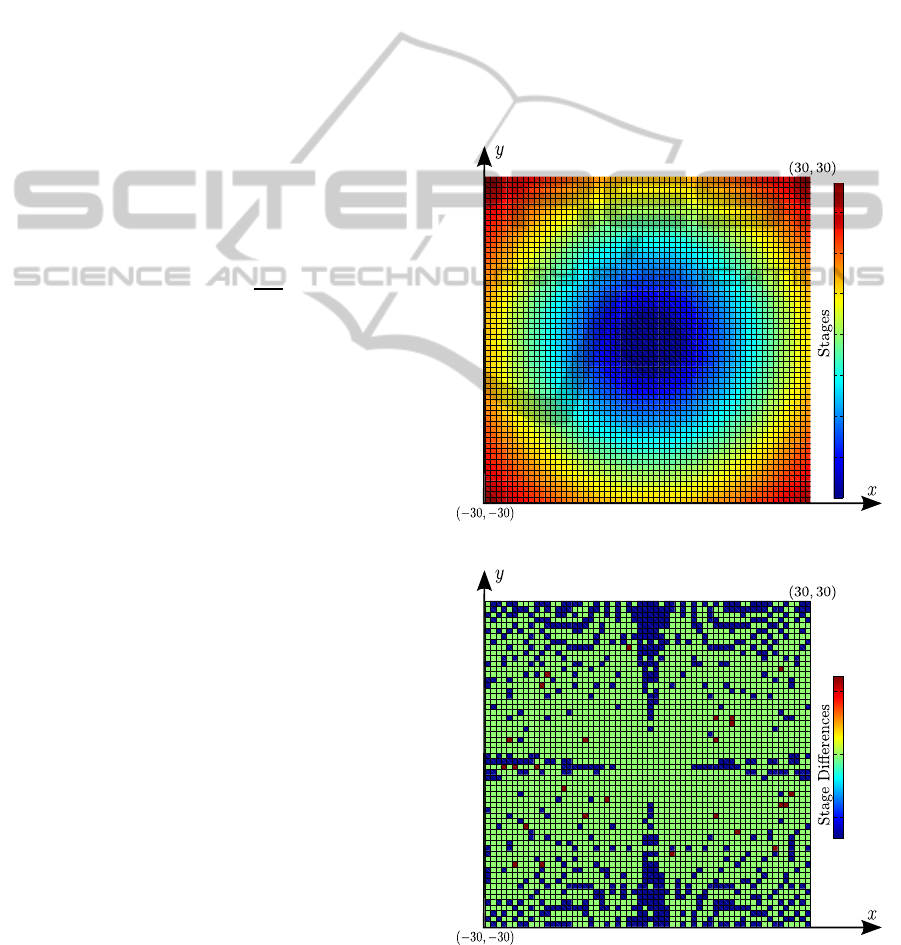
Figure 2(a) depicts the value function over the re-

garded discretized state space computed by the em-

bedded computer. Regarding this solutions the con-

vergence of the PEG in three dimensions is given

everywhere, meaning that in this conﬁguration the

evader can never avoid to be captured by the pur-

suer. Figure 2(b) depicts the difference of the value

of stages between the MATLAB simulation and the

simulation on the embedded computer. The differ-

ences are slightly in the whole state space. Moreover,

due to the very small differences (caused by possible

rounding errors and varieties in the minimization al-

gorithm implementation) between the MATLAB and

the embedded computer solution, the implementation

on the BeagleBone Black was accomplished success-

fully. The next important point was to check the real-

time applicability of the approach. The demanded

computational time of ∆T = 0.1s for one stage of

the game was successfully satisﬁed. By conﬁguring

the algorithm for the saddle-point computation of one

stage k, such that it stops after maximal 0.09s, the

minimization algorithm was still able to maintain the

demanded absolute tolerance of 10

−6

for the mini-

(a) Value of stages needed for capture.

-1

(b) Difference of value of stages needed for capture in MATLAB and on the

embedded computer.

Figure 2: Simulation Results.

ICINCO2014-11thInternationalConferenceonInformaticsinControl,AutomationandRobotics

mum function value. The use of an RTOS assures

that the algorithm yields a solution within ∆T = 0.1s,

thus the real-time speciﬁcations are satisﬁed.

8 CONCLUSIONS

The goal of this paper was to present a framework,

which enables the solution of a PEG with UAVs in

three dimensions. This framework, formulated in

a game-theoretical manner, does not only provide a

solution approach for the present problem, but for

all problems which can be formulated as N-player

discrete-time deterministic dynamic games. By ap-

plying this approach the convergence of the PEG in a

three-dimensional environmentwith UAV agents hav-

ing dynamic constraints was shown successfully. Fur-

thermore, the approach was implemented on an em-

bedded computer providing results equal to the MAT-

LAB implementation. Finally, the real-time applica-

bility of the approach was shown successfully in sim-

ulations. This paper forms the basis for a real UAV

system implementation of the presented approach,

which will be carried out next on the quad-rotor

system L4-ME of HiSystems GmbH (MikroKopter,

2014).

REFERENCES

Alexopoulos, A., Kandil, A. A., Orzechowski, P., and

Badreddin, E. (2013). A comparative study of col-

lision avoidance techniques for unmanned aerial vehi-

cles. In SMC, pages 1969–1974.

Bas¸ar, T. and Olsder, G. J. (1999). Dynamic Noncooperative

Game Theory (Classics in Applied Mathematics). Soc

for Industrial & Applied Math, 2 edition.

Beatty, M. (2006). Principles of Engineering Mechanics:

Volume 2 Dynamics – The Analysis of Motion. Math-

ematical Concepts and Methods in Science and Engi-

neering. Springer.

Bellman, R. (1957). Dynamic Programming. Princeton

University Press, Princeton, NJ, USA, 1 edition.

Bouabdallah, S. and Siegwart, R. (2007). Advances in Un-

manned Aerial Vehicles, chapter Design and Control

of a Miniature Quadrotor, pages 171–210. Springer

Press.

Chatterjee, B. (2009). An optimization formulation to com-

pute nash equilibrium in ﬁnite games. In Methods and

Models in Computer Science, 2009. ICM2CS 2009.

Proceeding of International Conference on, pages 1–

Chatterjee, B. (2010). n-person game.

www.mathworks.com/matlabcentral/ﬁleexchange/

27837-n-person-game.

Chung, T. H., Hollinger, G. A., and Isler, V. (2011). Search

and pursuit-evasion in mobile robotics. Autonomous

Robots, 31(4):299–316.

CubieTech Ltd. (2014). Cubieboard – A series of open

ARM miniPCs. www.cubieboard.org.

Isaacs, R. (1965). Differential Games: A Mathemati-

cal Theory with Applications to Warfare and Pursuit,

Control and Optimization. John Wiley and Sons, Inc.,

New York.

Johnson, S. G. (2013). The nlopt nonlinear-optimization

package. http://ab-initio.mit.edu/nlopt.

Kraft, D. (1988). A software package for sequential

quadratic programming. Technical Report DFVLR-

FB 88-28, DFVLR, Cologne, Germany.

Kraft, D. (1994). Algorithm 733: Tompfortran modules for

optimal control calculations. ACM Transactions on

Mathematical Software, 20(3):262–281.

Krstic, M., Kokotovic, P. V., and Kanellakopoulos, I.

(1995). Nonlinear and Adaptive Control Design. John

Wiley & Sons, Inc., New York, NY, USA, 1st edition.

LaValle, S. M. and Hutchinson, S. A. (1993). Game theory

as a unifying structure for a variety of robot tasks. In

Proceedings of 8th IEEE International Symposium on

Intelligent Control, pages 429–434. IEEE.

Littlewood, J. E. (1986). Littlewood’s Miscellany. Cam-

bridge University Press.

MikroKopter (2014). MK-QuadroKopter / L4-ME. http://

www.mikrokopter.de/ucwiki/MK-Quadro.

Nahin, P. J. (2012). Chases and Escapes: The Mathematics

of Pursuit and Evasion (Princeton Puzzlers). Prince-

ton University Press.

Nash, J. F. (1950). Non-cooperative Games. PhD thesis,

Princeton University, Princeton, NJ.

Raspberry Pi Foundation (2014). Raspberry Pi.

www.raspberrypi.org.

Sgall, J. (2001). Solution of david gale’s lion and man prob-

lem. Theoretical Computer Science, 259(1-2):663–

670.

Texas Instruments Inc. (2014a). Beagleboard.org.

www.bealgeboard.org.

Texas Instruments Inc. (2014b). BeagleBone Black.

www.beagleboard.org/Products/BeagleBone Black.

Thomas, L. C. (1984). Games, Theory and Applications.

Dover Books on Mathematics. Dover Publications.

Vieira, M., Govindan, R., and Sukhatme, G. (2009). Scal-

able and practical pursuit-evasion. In Robot Commu-

nication and Coordination, 2009. ROBOCOMM ’09.

Second International Conference on, pages 1–6.

von Neumann, J. and Morgenstern, O. (2007). Theory

of Games and Economic Behavior (60th-Anniversary

Edition). Princeton University Press.

Voos, H. (2009). Entwurf eines ﬂugreglers f¨ur ein vier-

rotoriges unbemanntes ﬂugger¨at (control systems de-

sign for a quadrotor uav). Automatisierungstechnik,

57(9):423–431.

APursuit-evasionGameBetweenUnmannedAerialVehicles