System Reactivity Components in Cellular Manufacturing Subjected
to Frequent Unavailability of Physical and Human Resources
Sameh M. Saad
1
and Carlos R. Gómez
2
1
Department of Engineering and Mathematics, Sheffield Hallam University, Sheffield, U.K.
2
Department of Materials, Mechanical and Manufacturing, Nottingham University, Nottingham, U.K.
Keywords: Cellular Manufacturing, Internal Disturbances, Simulation.
Abstract: In manufacturing systems, different types of disturbances influence system’s performance. In this paper
those components within a manufacturing cell contributing to maintain a higher performance, despite the
influence of internal disturbances such as machine breakdowns and operator unavailability, are investigated.
Discrete event simulation is used to model the processing and material handling subsystems within a
cellular manufacturing. Experimentation is conducted using a full factorial design and data analysis is
performed using analysis of variance. The results indicated that, in terms of systems reactivity, processing
subsystems aspects such as the skills of the operators, the capacity of the buffers and the duration of
machine set-ups are more efficient in coping with work-in-progress (WIP) resulting from the effect of
disturbances than aspects related to the material handling sub system.
1 INTRODUCTION
In a current economic environment characterised by
increasing uncertainty, manufacturing systems are
more vulnerable to the effects of unpredictable or
random events commonly referred to as
manufacturing disturbances. A particular type of
disturbances includes all the disrupting events
occurring within the limits of manufacturing
systems. These are known as internal disturbances
and are characterised by the limited availability of a
specific resource (Saad and Gindy, 1998). In order
to remain competitive in an environment of
uncertainty, it is necessary for manufacturing
systems to identify those components providing the
system with the capability to efficiently perform
under such disrupting conditions.
Manufacturing systems are determined by a
transformation process where inputs are converted
into outputs by means of an internal process. The
internal process is an assembly of interconnected
components (e.g. machines, material handling
devices and human resources) whose interaction
determines the outcome of the system. A cellular
system is a particular layout configuration of a
manufacturing system where different types of
machines are grouped together according to the
process combination occurring within a family of
parts. Among some benefits of cellular
manufacturing, Williams (1994) reported an
increased efficiency by reducing material handling
and transportation cost. Compared to other layout
configurations such as functional layouts, where
machines are grouped together based on similar
functions, cellular systems offer better results in
terms of work-in-process inventory, particularly
when there are small batches and short run times
involved (Logendran and Talkington, 1997).
Eckstein and Rohleder (1998) claimed that cellular
configurations also offer more advantages in terms
of human issues such as the operator’s learning rate
and the number of workers employed.
Modern manufacturing systems operate under
uncertain conditions originated within the
boundaries of the system; such internal conditions
range from uncertainty about processing times to
uncertainty about resources’ reliability. Having into
consideration that, for a considerable number of
organizations, it is prohibitive to acquire additional
capacity in order to guarantee a safe operation
against uncertainty, the only way for manufacturing
systems to meet deadlines is by using available
resources. Reactivity has been defined as the
capacity if the system to react to internal
disturbances and constitutes a significant aspect
373
Saad S. and R. Gómez C..
System Reactivity Components in Cellular Manufacturing Subjected to Frequent Unavailability of Physical and Human Resources.
DOI: 10.5220/0005038803730384
In Proceedings of the 4th International Conference on Simulation and Modeling Methodologies, Technologies and Applications (SIMULTECH-2014),
pages 373-384
ISBN: 978-989-758-038-3
Copyright
c
 2014 SCITEPRESS (Science and Technology Publications, Lda.)

regarding the evolution of manufacturing systems.
Reactivity, according to Ounnar and Ladet (2004),
is achieved by exploiting the flexibility of physical
resources.
On the one hand, processing machines are the
most pervasive physical resources in manufacturing
systems. On the other hand, the human element is
another physical resource mainly associated with
control tasks within such systems. Both types of
resources have received significant research
attention, particularly in issues regarding the
reactivity of manufacturing systems. Regarding
processing machines, one important aspect of system
reactivity is the capability of machines to efficiently
perform despite the presence of frequent
breakdowns, which is one of the most inherent
disturbances within systems’ limits. Dynamic
scheduling, where real time decisions are made in
order to offer a rapid response to disturbances, is one
of the most favoured approaches to cope with
machine breakdowns. Nihat et al. (2006) claimed
that it is possible to reduce the adverse impact of
machine breakdowns by using intelligent scheduling
policies that exploit available information about
sources of uncertainty. They proposed a stochastic
scheduling approach to characterize uncertainty
using probability distributions and generated optimal
policies under different distributional assumptions.
Ounnar and Ladet (2004) investigated reassignment
strategies and proposed a multi-criteria algorithm for
reassigning parts from a broken down machine into
an alternate machine and by considering the best
compromise between the variables time, cost and
machine reliability. Ozmutlu and Harmonosky
(2004) stated that conventional re-routing strategies
become more difficult to achieve as the complexity
of manufacturing system increase; therefore they
proposed a threshold –based selective rerouting
strategy to minimize the mean flow time in a system
with machine breakdowns. Their strategy achieved
superior results compared to other strategies and also
has the advantage of being simpler in its application.
Chen and Chen (2003) recognised that a frequent
rescheduling due to recurrent machine breakdowns
can make the behaviour of the system hard to
predict, reducing the effectiveness of dynamic
scheduling . To avoid this, the authors proposed
adaptive scheduling, which consist in updating the
job ready time and completion time, and the
machine status on a rolling horizon basis; they also
suggested considering machine availability in
generating schedules.
Other approaches to cope with machine
breakdowns look at the improvement of repair times
and facilities in order to reduce machine down time,
the implementation of preventive maintenance
policies to either avoid or reduce failures, the
consideration of wok-in-process inventory buffers as
a safety measure, etc (Buffa, 1972). Taylor et al.
(1982) used network modelling in order to analyse
alternative approaches for maintaining desired
levels of system output in the presence of machine
breakdowns. Hillier and So (1991) analysed the
effects of inter-stage storage on the performance of a
system subjected to machine breakdowns; they
concluded that, in the event of a machine
breakdown, a suitable inter-stage storage capacity
helps to provide parts for downstream machines,
reducing the effect of the disturbance. In a very
unconventional approach Liao and Chen (2004)
proposed maximising set-up time subject to a due
date constraint in order to reduce machine
breakdowns rate.
Concerning the human resource element of
manufacturing systems, aspects particularly related
to the level of skills and the extent of human
resource involvement in manufacturing processes,
have been investigated as determinants of system’s
reactivity.
Concerning the human element, it is clear that
despite increasing automation of manufacturing
systems, the human element is still an essential
component (Hwang et al., 1984). It has been
demonstrated that success in the implementation of
advanced manufacturing technology is due not to
technical failures but to human related issues such as
the capability of workers in terms of skills,
knowledge and attitude (Chung, 1996). In a study
carried out by Kahn and Lim (1998), the authors
found strong evidence that productivity growth was
increasingly concentrated in the more skill-intensive
manufacturing industries. Pagell et al. (2000)
pointed out that a key advantage of skilled workers
is their ability to more easily cope with increasing
complexity and uncertainty; however, the higher
costs associated to high skilled workers and the
dependence upon scarce resources can be
discouraging factors. This may just be the reason
why despite of the existing evidence on the
relationship between productivity and a skilled
workforce, a considerable number of manufacturing
organisations still rely on low skilled workers.
Regarding the fact of manufacturing systems and
their current uncertain environment, the link
between uncertainty and an increased need for more
flexible workers has been established. There is
extensive research focusing mostly on the impact of
human resource practices on the performance of
SIMULTECH2014-4thInternationalConferenceonSimulationandModelingMethodologies,Technologiesand
Applications
374

manufacturing systems. Among some of the relevant
research, Pagell et al. (2000) suggested that a poorly
developed human resource strategy often leads to
low performance levels in environments of advance
manufacturing technology. Huselid (1995)
investigated the impact of human resource
management practices, such as new skills
acquisition, on corporate financial performance. The
authors suggested that such practices lead to an
improved performance, particularly in terms of
employee turnover and productivity. Similarly,
Jayaram et al. (1999) also investigated the impact of
common human resource practices on a series of
performance measures, namely cost, quality,
flexibility and time. The authors found a strong
positive relationship between employee-skills
related factors and performance. Udo and Ebienfung
(1999) confirmed such relationship by investigating
the impact of human factors, such as employee
training, on performance indicators like ROE,
reduced cost, quick throughput , competitiveness,
control, response, improved condition and quality.
The purpose of this study is to understand how
the key components of a cellular manufacturing
system can contribute to system’s reactivity. In this
section, it has been mentioned that components such
as machines and human workers may possess
particular characteristics or abilities that make them
able to individually contribute to a better system
performance. In this study the technical aspect of
manufacturing systems, represented by machines
and material handling equipment, is combined with
the human aspect in order to identify those features
that provide the system with the capability to
perform under uncertain environments characterised
by frequent machine breakdowns and frequent
operator unavailability.
The objective of this study is achieved by using
discrete event simulation combined with statistical
design of experiments. Simulation has enabled the
representation of a complex manufacturing
environment and a full factorial design of
experiments has made possible the consideration of
the interactions occurring between all the
components within the defined system. As opposed
to other research on the topic of system reactivity,
this study looks at a combination of factors and
different experimental scenarios. This consideration
of a bigger picture enables a better understanding of
system reactivity and the alternative ways to achieve
it.
2 RESEARCH
METHODOLOGIES
2.1 Simulation Model
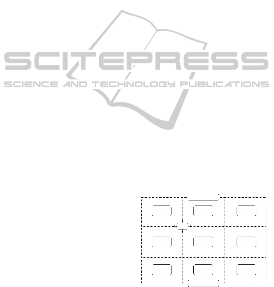
The cellular manufacturing system considered in this
paper consists of nine work centres. Each work
centre is composed of one input buffer, one
machine, and one output buffer. Parts arrive one at
time into the system following a representative
probability distribution. A loading area receives five
different types of parts corresponding to five
different products. As soon as ten parts of a
particular type are available in the loading area,
those parts are pushed into their corresponding
processing route. Each part type follows a specific
processing route with different processing times.
When a batch of parts is delivered to a work centre
the parts are directed into an input buffer first.
Afterwards, a machine operator collects one part
from the input buffer and loads it into the machine
for its processing. The operator stays next to a
machine during the whole machine processing time.
Once the machine finishes processing the part the
operator takes the part and places it into an output
buffer. Both the machine and the operator become
available for the next part to be processed. Parts
placed in output buffers are ready to be taken to the
following work centre along the processing route.
The flow of parts between the work centres is
assisted by an AGV based material handling system.
After parts have gone through all the processes
along the route they are delivered to an unloading
area from where they are subsequently shipped to
customers. The described manufacturing system is
represented in figure 1.
Figure 1: Manufacturing system layout.

Workcentre
1
Workcentre
2
Workcentre
3
Workcentre
6
Workcentre
5
Workcentre
4
Workcentre
7
Workcentre
8
Workcentre
9
Loadingarea
Unloadingarea
AGV
SystemReactivityComponentsinCellularManufacturingSubjectedtoFrequentUnavailabilityofPhysicalandHuman
Resources
375

2.2 Operating Assumptions
The system represented in figure 1 operates under
the following assumptions:
2.2.1 Parts
 Parts arrive in the system one at a time and
following an exponential distribution with an
average inter-arrival time of 45 minutes. The
exponential distribution has been selected
because of the existing resemblance between
such distribution and the inter arrival times for
real world systems (Law and Kelton, 2000).
 There are five different products involved; each
product with different processing requirements,
i.e. different processing times and routes. Process
routing is fixed for each of the products.
2.2.2 Machines
 Each machine represents a specific
manufacturing process within the system; they
can process only one piece at a time.
 Although all of the machines are assumed to
follow a normal distribution in both processing
and set up times, the times are different from
each other.
 There is a different usage cost per minute
associated with each machine.
 Machines do not have any automation level,
therefore each machine do require an operator.
 It is assumed that all machines breakdown from
time to time, consequently a different efficiency
level has been predefined for each machine.
 When machines fail, repairs are assumed to be
carried out by external personnel (not considered
for the purposes of this research). Machine
repairs are assumed to follow an exponential
distribution with different average times for each
machine.
2.2.3 Buffers
 Blocking does not occur.
 Buffer capacity is limited; all the buffers have
the same capacity. There is a storage cost per
item per minute associated with the capacity, i.e.
the higher the capacity the higher the storage
cost.
 Parts in buffers are prioritized according to FIFO
dispatching rule, i.e. parts are dispatched either
into a machine or vehicle considering a first
come first served rule.
2.2.4 Operators
 Operators have different abilities; in
consequence labour cost is associated with the
skill level.
 Operators are assumed not to be always
available, therefore different availability
percentages and absence times have been
specified for each operator.
 Travelling times for operators have not been
considered.
2.2.5 Automated Guided Vehicle
 The material handling system is totally
independent from human operators.
 The AGV travels at a constant speed along a
fixed route connecting all the work centres.
 Material handling costs are omitted and no
vehicle breakdowns are assumed.
 The AGV’s travelling time is determined based
on its speed.
2.3 Model Verification
Model verification can be carried out in three
different and complementary ways: Checking the
code, performing visual checks, and inspecting
output reports (Robinson, 1994). Code checking was
facilitated by the capabilities of the simulation
software, which made possible to interactively check
the coding line by line. Visual checks were
performed by keeping track of parts progressing
throughout the system, allowing the behaviour of all
the components intervening along the process to be
monitored. Additionally, the model was run in an
event-by-event mode in order to complement the
verification process.
This verification procedure made possible to
guarantee that each element within the model would
behave as it was originally intended. The last
method of model verification consisted in checking
the outputs of the main components within the
model; to do so 30 replications, each with a run time
of 400 simulation-hours, were conducted. After
analysing some of the most important system
outputs it was possible to confirm that all the model
components performed according to what had been
defined during the model coding process.
2.4 Model Validation
Model validation provides the confidence during the
experimentation stage and is basically concerned
with the extent to which a certain model is
SIMULTECH2014-4thInternationalConferenceonSimulationandModelingMethodologies,Technologiesand
Applications
376

representative of a real system. The level of
representation will be judged upon the viability of
making decisions based on the information provided
by the simulation model. Ideally, a model would be
better validated when compared to a real system
(Pidd, 1993); however, models do not always
represent real systems. Because the latter is the case
in the present research, it was not necessary to
compare the model with either empirical data or the
behaviour of a real system (Maki and Thompson,
2006).
Validation techniques are classified in two
groups, namely subjective techniques and objective
techniques. Objective validation-techniques do
require the existence of real systems in order to
establish input-output comparisons between systems.
Subjective techniques, as their name imply, does not
necessarily require the existence of a real system
since they are more dependent on the experience and
“feelings” of its developers (Banks, 1998). The
proposed model has been validated using a
sensitivity analysis as a subjective validation
method. The sensitivity analysis capability is a built-
in feature in Simul8; its function is to test the
assumed probability distributions in terms of how
sensitive the results are to changes in these inputs. A
number of probability distributions particularly
related to machine processing times and set-ups have
been randomly selected to be tested. The sensitivity
analysis confirmed the validity of the assumptions.
3 EXPERIMENTAL DESIGN
The experimental design of this study was concerned
with:
(i) Selecting the response variables;
(ii) Determining the model running time;
(iii) Choosing the experimental factors and
settings; and
(iv) Defining the statistical design of the
experiments.
3.1 Selection of Response Variables
The performance of the investigated manufacturing
system was measured in terms of three
complementary response variables, namely number
of completed parts, manufacturing cost, and average
time in the system.
3.2 Model Running Time
In a simulation model, the total running time
consists of a warming-up period, during which the
model reaches normal operating conditions, and a
run length period, during which the model collects
results. In order to determine the model warm-up
period Welch’s graphical method was used. In this
method, the model will be run several times with
different random number seeds in order to calculate
a mean average of a key output for specific periods
of time, afterwards moving averages are calculated
(Robinson, 1994). For the proposed model, Welch’s
method indicated a minimum warm-up period of 50
hours (Welch, 1983).
On the other hand, the run length period of the
simulation model was determined by means of
another graphical approach described by Robinson
(1994). According to such approach, a minimum run
length period of 220 hours was required to gather
enough data.
3.3 Experimental Factors
Considering that this study has a special interest in
the physical components of manufacturing systems,
the design factors were grouped in aspects
concerning the two main subsystems in the model,
i.e. work centres and the handling of material. See
Table 1 below.
Table 1: Design factors.
Subsystem
Aspect
(Design factor)
Definition
Work centre
The skill level
of operators
It is determined by the
number of different
machines a single
operator can control.
The capacity of
buffers
It is related to the
maximum number of
parts the system is able to
hold.
The duration of
machine
set-ups
It is the time it takes for
machines to switch from
producing one type of
part to producing a
completely different part.
Material
handling
system
The number of
AGVs
It is related to the total
number of material
handling vehicles within
the system.
The speed of
AGVs
It is the distance covered
by material handling
vehicles during a specific
period of time.
The loading
capacity of
AGVs
The maximum number of
parts a material handling
vehicle can transport
between work centres.
SystemReactivityComponentsinCellularManufacturingSubjectedtoFrequentUnavailabilityofPhysicalandHuman
Resources
377

4 MODELS SCENARIOS
In order to reflect the effects of internal disturbances
and taking into consideration technological and
human resources, two different noise factors were
considered, namely an increase of machine
breakdowns and an increase in operator
unavailability. See Table 2 below for a definition of
each disturbance scenario.
Table 2: Internal disturbances.
Disturbance Definition
Machine
breakdowns
The purpose of this scenario is to
identify system components
contributing to maintain a higher
performance when there are recurrent
failures in machines throughout the
system. It is widely known that when
a manufacturing system does not have
the capability to cope with frequent
machine breakdowns, the system will
eventually come to a stop as a result
of increasingly accumulating WIP
inventory.
To simulate this scenario, the
original machine efficiencies, ranging
between 83% and 96%, have been
decreased. The new machine
efficiencies ranging between 60% and
70% have been randomly assigned to
each machine within the system.
Operator
unavailability
In this scenario, the system is subject
to long unavailability periods of
human operators in order to identify
suitable system’s responses. In a
similar way to the previous scenario,
the unavailability of human resources
for long periods of time can
significantly affect performance by
interrupting the production flow along
the system.
To simulate this scenario original
operator availability percentages have
been decreased from a range between
96% and 97% to a range between
91% and 95%. The average absence
time per operator ranges from 480 to
600 minutes. Both availability
percentages and absence times are
randomly assigned to operators.
There is a direct relationship between these two
scenarios given that both are characterised by the
unavailability of a specific resource during a period
of time; however, the aim of each scenario is
different since two different aspects of resource
unavailability are examined. The machine
breakdowns scenario examines the aspect of
frequency of unavailability, whereas the scenario of
operator unavailability examines the aspect of the
duration of resource unavailability.
4.1 Factor Levels and Range
The objective of the experiment is to identify the
factors with a higher influence on the response
variable, it is recommended to keep a low number of
factor levels, with a relatively large range between
levels (Montgomery, 2009). After establishing and
testing a series of ranges for each of the considered
factors, the levels and ranges shown in Tables 3 and
4 were chosen for the factors in the two considered
scenarios.
Note that factor levels are different in both tables
because each table corresponds to a specific scenario
where the effect of a particular disturbance was
analysed before choosing adequate factor levels.
4.2 Number of Necessary Replications
The number of necessary replications for each
simulation scenario was determined by calculating a
maximum error estimate out of a series of initial
model replications. The maximum error estimate
together with a desired error was taken into account
to determine the required number of replications for
each model. According to such calculation, a
minimum of 250 replications per model were
enough to guarantee statistical reliability at a 95%
confidence interval.
4.3 Data Structuring and Analysis
The simulation experiments were conducted
according to a complete factorial experimental
design , which was a suitable design due to the fact
that possible factor interactions needed to be
considered (Mason et al., 2003). Considering that
there were 6 design factors involved, each at two
levels, a 2
6
full factorial design was employed.
Given the high variation in the resulting data related
to the responses cost and time, the original data has
been normalized using a log transformation.
Subsequently an analysis of variance was conducted
to identify the significant factors. Main effects plots
and interaction plots were used to identify factor
levels and factor interactions respectively. Minitab
was the statistical software used to analyse the data
provided by each simulation scenario.
SIMULTECH2014-4thInternationalConferenceonSimulationandModelingMethodologies,Technologiesand
Applications
378

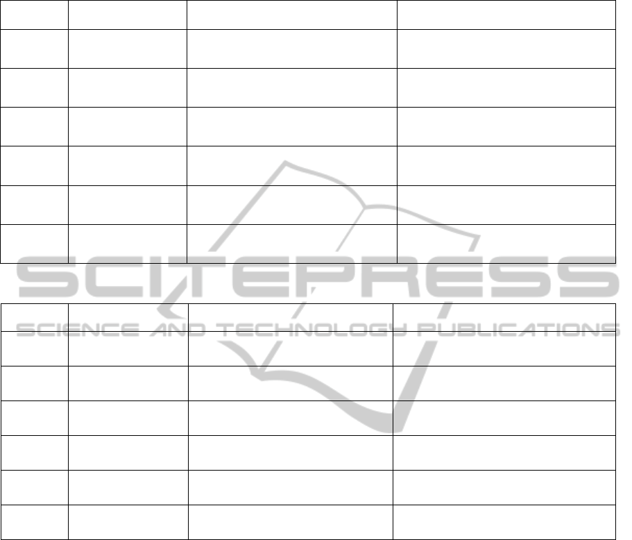
Table 3: Frequent machine breakdowns scenario: Factor levels.
FACTOR DESCRIPTION LEVEL 1 LEVEL 2
A
Operator skills
4 unskilled operators and 2 semi-
skilled operators.
3 semi-skilled operator and 3 skilled
operators
B
Buffer capacity
Buffer capacity of up to 10 parts; cost
per item per minute $0.010.
Buffer capacity of up to 29 parts; cost
per item per minute $0.030.
C
Number of vehicles 1 AGV. 4 AGVs.
D
Vehicle speed Vehicle speed 5 km/hr. Vehicle speed 60 km/hr.
E
Loading capacity of
AGV
3 parts loading capacity. (load/unload
= 0.5 min)
10 pieces loading capacity (load/unload
= 1.2 min)
F
Machine set-ups
duration
Set-up time between 1 and 5 minutes. Set-up time between 20 and 29 minutes.
Table 4: Frequent operator unavailability scenario: Factor levels.
FACTOR DESCRIPTION LEVEL 1 LEVEL 2
A
Operator skills
4 unskilled operators and 2 semi-
skilled operators.
2 semi-skilled operator and 4 skilled
operators.
B
Buffer capacity
Buffer capacity of up to 10 parts; cost
per item per minute $0.010.
Buffer capacity of up to 29 parts; cost
per item per minute $0.030.
C
Number of vehicles 1 AGV. 5 AGVs.
D
Vehicle speed Vehicle speed 5 km/hr. Vehicle speed 80 km/hr.
E
Loading capacity of
AGV
4 parts loading capacity.
(load/unload = 0.5 min)
10 pieces loading capacity (load/unload
= 1.2 min)
F
Machine set-ups
duration
Set-up time between 6 and 10
minutes.
Set-up time between 20 and 29 minutes.
5 ANALYSIS AND RESULTS
5.1 Machine Breakdowns Scenario
The analysis of variance of the results, in terms of
each of the three considered response variables, has
been calculated for this scenario. Tables 5, 6, and 7
show the ANOVA tables for the responses number
of parts, cost, and average time in the system
respectively. Note that the statistical package used to
analyse the results – Minitab – automatically omits
those main factors whose direct contribution to the
response is not significant. For this reason the factor
vehicle speed is not included in Table5 and the
factor loading capacity is not considered in Tables 6
and 7.
Table 5: ANOVA table for the response number of parts.
Source DF SS MS F P
Operators skills 1 0.60567 0.60567 11.03 0.002*
Buffer capacity 1 2.15831 2.15831 39.30 0.000*
Number of vehicles 1 0.00838 0.00838 0.15 0.698
Loading capacity 1 0.11816 0.11816 2.15 0.149
Set up duration 1 0.05766 0.05766 1.05 0.311
Operators skills*Loading capacity 1 0.47699 0.47699 8.69 0.005*
Operators skills*Buffer capacity 1 0.27227 0.27227 4.96 0.031
Operators skills*Number of vehicles 1 0.00296 0.00296 0.05 0.818
Buffer capacity*Number of vehicles 1 0.06154 0.06154 1.12 0.295
Buffer capacity*Loading capacity 1 0.00439 0.00439 0.08 0.779
Buffer capacity*Set up duration 1 0.00152 0.00152 0.03 0.868
Loading capacity*Set up duration 1 0.00197 0.00197 0.04 0.851
Operators skills*Buffer capacity* 1 0.35865 0.35865 6.53 0.014*
Number of vehicles
Buffer capacity*Loading capacity* 1 0.37574 0.37574 6.84 0.012*
Set up duration
Error 49 2.69103 0.05492
Total 63 7.19523
S
= 0.234348 R
-
S
q = 62.60% R
-
S
q(adj) = 51.91%
SystemReactivityComponentsinCellularManufacturingSubjectedtoFrequentUnavailabilityofPhysicalandHuman
Resources
379

Table 6: ANOVA table for the response cost.
Table 7: ANOVA table for the response time.
In Tables 5, 6, and 7, low p-values, at alpha =
0.05, identify those important main factors and
interactions. To make the identification easier,
significant factors and interactions have been
marked with a *. Even though the analysis of
variance identified significant factors and
interactions, it was necessary to confirm their level
of significance by looking at the percentage of
contribution of each factor and factor interaction.
Percentage of contribution is an indication of the
weight of each factor and factor interaction in
relation to the response variable; Percentage of
contribution calculation is part of Minitab’s
capabilities. Table 8 below shows these calculations
of the identified significant factors and interactions
as calculated by Minitab.
See Table 8 for the percentage of contributions
of the important factors and interactions to the
related response variable.
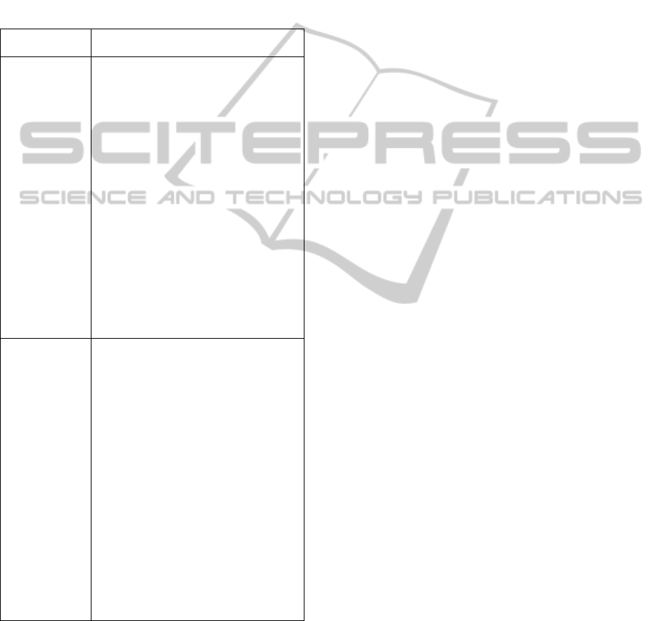
Regarding the response number of completed
parts, the information presented in Table 8 confirms
the results presented previously in Table 5. From
upper left section of Table 8, it can be noticed that
the combined percentage of contribution of the
factors operators’ skills and buffer capacity was of
approximately 39%. Additionally, the contribution
of the two significant interactions adds up to slightly
over 10%. As evidenced by the main effect plot in
the lower left section of Table 8, buffer capacity at
the highest level was the most important factor in
terms of number of completed parts; operators’ skill
at the lowest level was the second important factor.
Concerning the response cost, the percentage
contribution section at the upper middle section of
the table shows that only two out of the four
important factors identified in Table 6 were in fact
significant; those were buffer capacity and set-up
duration, both with a combined percentage
contribution of approximately 98%. Interaction’s
contribution was negligible. The main effect plot at
the lower middle of the table shows that buffer
capacity at its lowest level was the most significant
factor followed by set-up duration at its lowest level.
In relation to the response time in the system, the
percentage contribution section at the upper right
corner of Table 8 confirms that only 2 out of the
originally 4 identified important factors were
actually significant; those were operators’ skills and
set-up duration, both with a combined percentage
contribution of approximately 93%. No significant
interactions were presented. The main effects plot in
the lower right section of Table 8 indicates that the
factor operators’ skills at its highest level and set-up
duration at its lowest level were the only significant
factors in terms of a minimum time in the system.
5.2 Operator Unavailability
Similarly to the previous scenario, Minitab
automatically excluded those insignificant factors in
the analysis of variance, which are presented in
Tables 9, 10 and 11 below.
Table 8: ANOVA table for the response number of parts.
Source DF SS MS F P
Operators skills 1 0.002607 0.002607 1397.28 0.000*
Buffer capacity 1 0.487377 0.487377 261253.72 0.000*
Number of vehicles 1 0.000016 0.000016 8.52 0.005*
Vehicle speed 1 0.000002 0.000002 1.18 0.282
Set up duration 1 0.035603 0.035603 19084.53 0.000*
Operators skills*Buffer capacity 1 0.006888 0.006888 3692.30 0.000*
Operators skills*Number of vehicles 1 0.000022 0.000022 11.69 0.001*
Operators skills*Set up duration 1 0.000383 0.000383 205.40 0.000*
Buffer capacity*Number of vehicles 1 0.000038 0.000038 20.25 0.000*
Buffer capacity*Vehicle speed 1 0.000011 0.000011 5.66 0.022
Buffer capacity*Set up duration 1 0.000389 0.000389 208.40 0.000*
Number of vehicles*Vehicle speed 1 0.000000 0.000000 0.19 0.669
Number of vehicles*Set up duration 1 0.000103 0.000103 55.25 0.000*
Vehicle speed*Set up duration 1 0.000107 0.000107 57.50 0.000*
Operators skills*Buffer capacity* 1 0.000290 0.000290 155.68 0.000*
Set up duration
Buffer capacity*Vehicle speed* 1 0.000013 0.000013 6.93 0.011
Set up duration
Number of vehicles*Vehicle speed* 1 0.000048 0.000048 25.52 0.000*
Set up duration
Error 46 0.000086 0.000002
Total 63 0.533982
S = 0.00136584 R-Sq = 99.98% R-Sq(adj) = 99.98%
Source DF SS MS F P
Operators skills 1 0.0612929 0.0612929 8727.27 0.000*
Buffer capacity 1 0.0013389 0.0013389 190.64 0.000*
Number of vehicles 1 0.0000364 0.0000364 5.18 0.028
Vehicle speed 1 0.0014422 0.0014422 205.34 0.000*
Set up duration 1 0.0597981 0.0597981 8514.42 0.000*
Operators skills*Buffer capacity 1 0.0014947 0.0014947 212.82 0.000*
Operators skills*Number of vehicles 1 0.0002010 0.0002010 28.61 0.000*
Operators skills*Vehicle speed 1 0.0001284 0.0001284 18.28 0.000*
Operators skills*Set up duration 1 0.0030511 0.0030511 434.43 0.000*
Buffer capacity*Number of vehicles 1 0.0000356 0.0000356 5.07 0.029
Buffer capacity*Vehicle speed 1 0.0000016 0.0000016 0.22 0.640
Buffer capacity*Set up duration 1 0.0001578 0.0001578 22.48 0.000*
Number of vehicles*Vehicle speed 1 0.0001291 0.0001291 18.38 0.000*
Number of vehicles*Set up duration 1 0.0003161 0.0003161 45.01 0.000*
Vehicle speed*Set up duration 1 0.0003820 0.0003820 54.39 0.000*
Operators skills*Buffer capacity* 1 0.0000464 0.0000464 6.61 0.014
Number of vehicles
Operators skills*Buffer capacity* 1 0.0002124 0.0002124 30.24 0.000*
Set up duration
Operators skills*Number of vehicles*1 0.0000465 0.0000465 6.61 0.014
Set up duration
Number of vehicles*Vehicle speed* 1 0.0001051 0.0001051 14.97 0.000*
Set up duration
Error 44 0.0003090 0.0000070
Total 63 0.1305251
S = 0.00265012 R-Sq = 99.76% R-Sq(adj) = 99.66%
Source DF SS MS F P
Operator skills 1 72.740 72.740 209.35 0.000*
Buffer capacity 1 50.297 50.297 144.76 0.000*
Number of vehicles 1 3.038 3.038 8.74 0.005*
Loading capacity 1 0.869 0.869 2.50 0.119
Operator skills*Buffer capacity 1 30.792 30.792 88.62 0.000*
Operator skills*Loading capacity 1 2.858 2.858 8.22 0.006*
Error 57 19.805 0.347
Total 63 180.398
S = 0.589452 R-Sq = 89.02% R-Sq(adj) = 87.87%
SIMULTECH2014-4thInternationalConferenceonSimulationandModelingMethodologies,Technologiesand
Applications
380

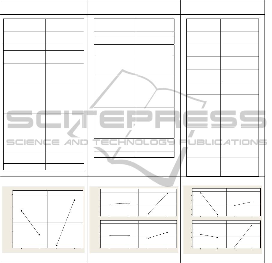
Table 9: Significant factors and factors interactions in terms of three response variables; machine breakdowns.
Number of completed parts Cost Time in the system
Model term
Percentage of
contribution
Operators’
skills
8.46 %
Buffer capacity 29.97%
Rest of main
factors
2.3%
Operators’
skills*Loading
capacity
6.66%
Operators’
skills*Buffer
capacity*Numb
er of vehicles
5.01%
Buffer
capacity*Loadi
ng
capacity*Set-up
duration
5.21%
Rest of
interactions
42.39%
Total 100%
Model term
Percentage of
contribution
Buffer capacity 91.27%
Set-up duration 6.67%
Rest of main
factors
0.49%
Operators’
skills*Buffer
capacity
1.29%
Operators’
skills*Set-up
duration 0.07%
Buffer
capacity*Set-up
duration 0.07%
Rest of
interactions
0.14%
Total 100%
Model term
Percentage of
contribution
Operators’
skills
46.96%
Buffer
capacity
1.03%
Vehicle
speed
1.10%
Set-up
duration
45.81%
Rest of
main factors
0.03%
Operators’
skills*Buffe
r capacity 1.15%
Operators’
skills*set-up
duration 2.34%
Rest of
interactions
1.58%
Total 100%
Table 10: ANOVA table for the response cost. Table 11: ANOVA table for the response time.
1-1
667.3
667.2
667.1
667.0
666.9
1-1
Operators skills
Mean
Buffer capacity
D
a
t
a
M
e
a
n
s
1-1
60000
55000
50000
45000
40000
1-1
1-1
60000
55000
50000
45000
40000
1-1
Operators skills
Mea n
Buffer capacity
Number of vehicles Set up duration
1-1
1700
1650
1600
1550
1500
1-1
1-1
1700
1650
1600
1550
1500
1-1
Operators skills
Mean
Buffer capacit y
Vehicle speed Set up duration
Source DF SS MS F P
Operator skills 1 0.002513 0.002513 390.45 0.000*
Buffer capacity 1 0.492206 0.492206 76469.78 0.000*
Set up duration 1 0.011401 0.011401 1771.32 0.000*
Operator skills*Buffer capacity 1 0.009631 0.009631 1496.23 0.000*
Operator skills*Set up duration 1 0.000157 0.000157 24.41 0.000*
Buffer capacity*Set up duration 1 0.000067 0.000067 10.45 0.002*
Error 57 0.000367 0.000006
Total 63 0.516343
S = 0.00253705 R-Sq = 99.93% R-Sq(adj) = 99.92%
Source DF SS MS F P
Operator skills 1 0.076130 0.076130 4999.58 0.000*
Buffer capacity 1 0.003489 0.003489 229.15 0.000*
Number of vehicles 1 0.000091 0.000091 5.97 0.018
Vehicle speed 1 0.002846 0.002846 186.90 0.000*
Set up duration 1 0.018487 0.018487 1214.06 0.000*
Operator skills*Buffer capacity 1 0.003524 0.003524 231.40 0.000*
Operator skills*Number of vehicles 1 0.000357 0.000357 23.44 0.000*
Operator skills*Set up duration 1 0.000954 0.000954 62.64 0.000*
Number of vehicles*Vehicle speed 1 0.000325 0.000325 21.33 0.000*
Vehicle speed*Set up duration 1 0.000158 0.000158 10.37 0.002*
Error 53 0.000807 0.000015
Total 63 0.107168
S
= 0.00390223 R
-
S
q = 99.
2
5% R
-
S
q(adj) = 99.10%
SystemReactivityComponentsinCellularManufacturingSubjectedtoFrequentUnavailabilityofPhysicalandHuman
Resources
381

Note that in this scenario the models generated by
the analysis of variance were much less complex
than the models in the first scenario, i.e. the models
had fewer terms in each of the considered responses.
The analysis of variance has preliminarily
identified a series of important factors and factor
interactions. By looking at the information presented
in Table 12 it is possible to confirm the real
significance of those factors in terms of the three
considered response variables.
The upper left section in Table 12 indicates that,
in terms of the response number of completed parts,
the only two significant factors were operators’
skills and buffer capacity; both with a combined
percentage of contribution of approximately 68%.
No significant interactions were present. The plot of
main effects in the lower left section shows that
these two factors were both significant at their
highest level.
In the column related to the response variable
cost, the upper middle section of Table 12 shows
that there was only one significant factor out of the
three originally identified factors. The factor buffer
capacity on its own had a percentage of contribution
to the response of approximately 95%. Compared to
this contribution, the other factors together with all
of the interactions cannot be considered significant.
The effects plot in the lower middle of Table 12
indicates that the factor buffer capacity was
significant at its lowest level.
In terms of the response time in the system, the
upper right section of Table 12 indicates that only 2
out of the originally identified important factor were
considerably significant; those were operators’ skills
and set-up duration. No significant factor
interactions were present in the model. The effects
plot in the lower middle section shows that the main
factor operators’ skill was significant to the response
at its highest level, whereas the main factor set-up
direction was significant at its lowest level.
6 DISCUSSION AND FUTURE
WORK
From the results section it can be noticed that,
although the level of significance may differ, the
significant factors are similar in both scenarios.
Regarding the response variable number of
completed parts, in the model with frequent machine
breakdowns the two most important factors were a
high buffer capacity in the first place and low
operators’ skills in the second place. This result
indicates that in a manufacturing environment
characterised by recurrent machine breakdowns a
higher buffer capacity to accommodate the excess of
WIP inventory accumulated during machine down
periods is the most desirable feature. According to
Hillier and So (1991), additional buffer space
reduces the adverse effect of machine breakdowns
and increases the throughput of the line.
Additionally, low skilled operators are more likely
to be dedicated to only one or two machines; this
guarantees the availability of the operator even when
the machine is down.
In the model characterized by a more frequent
rate of operator unavailability, the most important
and second most important factors were high
operators’ skills and high buffer capacity
respectively. In this type of environments, counting
on skilled operators is much more important than
relying on a high buffer capacity because skilled
operators can take on any machine when other
operators are absent during considerable periods of
time. A high buffer capacity, similarly to the
machine breakdowns scenario, contributes to
increase the throughput.
Concerning the response variable cost, both
scenarios indicated low buffer capacity as the most
important factor followed by low set-up duration.
Considering that the different processes along
cellular systems are accountable for WIP inventories
(Srinivasan and Bozer, 1992), an important approach
to keep costs down is to control the levels of costly
WIP inventories along the system. In order to
achieve this, the use of low capacity inter-storage-
areas to limit the size of WIP is an important first
step. In addition, a second important step to control
WIP levels and therefore maintain lower costs in
manufacturing environments characterized by the
temporary unavailability of resources is the
consideration of set-up reduction strategies.
In relation to the response variable time, the two
most important factors in each considered scenario
were high operator skills, in the first place, followed
by low set-up duration. Under a time minimization
criterion, the priority in both scenarios is to keep
parts flowing throughout the system and high skilled
operators, able to handle different processes, are the
solution to maintain a smooth production flow. Set-
up time reduction is also decisive for total
production lead time reduction (Dimitrov, 1990).
Low set-up durations contribute to maintain
production flow by keeping low levels of WIP and
compensating the time lost during periods of
resource unavailability.
SIMULTECH2014-4thInternationalConferenceonSimulationandModelingMethodologies,Technologiesand
Applications
382

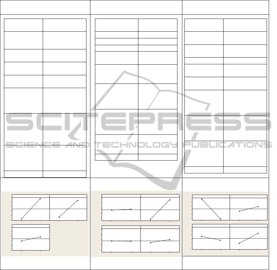
Table 12: Significant factors and factor interactions in terms of three response variables; operator unavailability.
Number of completed parts Cost Time in the system
Model term
Percentage of
contribution
Operators’
skills
40.31%
Buffer
capacity
27.88%
Number of
vehicles
1.69%
Rest of main
factors
1.17%
Operators’
skills*Buffer
capacity
17.06%
Operators’
skills*Loadin
g capacity 1.59%
Rest of
interactions
10.3%
Total 100%
Model term
Percentage of
contribution
Operators’ skills 0.49%
Buffer capacity 95.33%
Set-up duration 2.21%
Rest of main
factors
0.01%
Operators’
skills*Buffer
capacity
1.86%
Operators’
skills*Set-up
duration
0.03%
Buffer
capacity*Set-up
duration
0.01%
Rest of
interactions 0.06%
Total 100%
Model term
Percentage of
contribution
Operators’
skills
71.04%
Buffer
capacity
3.26%
Vehicle speed 2.66%
Set-up
duration
17.25%
Rest of main
factors
0.12%
Operators’
skills*Buffer
capacity
3.29%
Operators’
skills*set-up
duration
0.89%
Rest of
interactions
1.49%
Total 100%
In both disturbance scenarios, aspects related to the
processing subsystem of the manufacturing cell,
such as the skill level of the operators, the capacity
of buffers and the duration of machine set-up were
determinant to control the level of WIP inventories
within the system, which in turn was translated into
a system’s capacity to maintain a higher
performance. The only aspect related to the material
handling subsystem that appeared to be more
important, particularly for the response time, was the
speed of the vehicle. Similarly to the indentified
significant factors, vehicle speed is strongly linked
with WIP reduction (Srinivasan and Bozer, 1992).
No other of the aspect concerning the material
handling subsystem was considerably significant.
In addition to the consideration of system’s
reactivity, where manufacturing system’s behaviour
under the effect of internal disturbances is analysed,
the effect of external disrupting forces like those
related to the market could also be investigated.
Furthermore, both internal and external disturbances
could be investigated in the context of
manufacturing flexibility. By adopting a more
inclusive approach on the analysis of manufacturing
flexibility and the effect of disturbances, those
particular system components providing the system
1-1
667.0
666.5
666.0
665.5
665.0
1-1
1-1
667.0
666.5
666.0
665.5
665.0
Operator skills
Mean
Buffer capacity
Number of vehic les
D
a
t
a
M
e
a
n
s
1-1
60000
55000
50000
45000
40000
1-1
1-1
60000
55000
50000
45000
40000
1-1
Operator skills
Mean
Buf fer capacity
Vehicle speed Set up duration
1-1
1550
1500
1450
1400
1350
1-1
1-1
1550
1500
1450
1400
1350
1-1
Operator skills
Mean
Buffer capacity
Vehicle speed Set up duration
D
a
t
a
M
e
a
n
s
SystemReactivityComponentsinCellularManufacturingSubjectedtoFrequentUnavailabilityofPhysicalandHuman
Resources
383

with flexibility capabilities under a number of
disrupting situations could be identified. The
identification of such components could lead to a
number of system configurations, especially able to
absorb the effects of several disturbances.
REFERENCES
Buffa, E. S., 1972, Operations Management: Problems
and models, New York, Wiley.
Chen, J. & Chen, F., 2003, Adaptive scheduling in random
flexible manufacturing systems subject to machine
breakdowns. International Journal of Production
Research, 41, 1927-1951.
Chung, C., 1996, Human issues influencing the successful
implementation of advanced manufacturing
technology. Journal of Engineering and Technology
Management, 13, 283-299.
Dimitrov, P., 1990, The impact of flexible manufacturing
systems (FMS) on inventories. Engineering Costs and
Production Economics, 19, 165-174.
Eckstein, A. & Rohleder, T., 1998, Incorporating human
resources in group technology/cellular manufacturing.
International Journal of Production Research, 36,
1199-1222.
Hillier, F. & So, K., 1991, The effect of Machine
breakdowns and interstage storage on the performance
of production line systems. International Journal of
Production Research, 29, 2043-2055.
Huselid, M. A., 1995, The impact of human-resource
management-practices on turnover, productivity, and
corporate financial performance. Academy of
Management Journal, 38, 635-672.
Hwang, S. L., Barfield, W., Chang, T. C. & Salvendy, G.,
1984, Integration of humans and computers in the
operation and control of flexible manufacturing
systems. International Journal of Production
Research, 22, 841-856.
Jayaram, J., Droge, C. & Vickery, S. K., 1999, The impact
of human resource management practices on
manufacturing performance. Journal of Operations
Management, 18, 1-20.
Kahn, J. A. & Lim, J. S., 1998, Skilled labor-augmenting
technical progress in US manufacturing. Quarterly
Journal of Economics, 113, 1281-1308.
Law, A. & Kelton, D., 2000, Simulation Modelling and
Analysis, Singapore, McGraw-Hill.
Liao, C. J. & Chen, W. J., 2004, Scheduling under
machine breakdown in a continuous process industry.
Computers and Operations Research, 31, 415-428.
Logendran, R. & Talkington, D., 1997, Analysis of
cellular and functional manufacturing systems in the
presence of machine breakdown. International Journal
of Production Economics, 53, 239-256.
Mason, R., Gunst, R. & Hess, J., 2003, Statistical design
and analysis of experiments, with applications to
engineering and science, New York, Wiley-
Interscience.
Montgomery, D. C., 2009, Design and analysis of
experiments, Hoboken, NJ, John Wiley & Sons.
Nihat, K., Haldun, A. & Anand, P., 2006, Minimizing
makespan on a single machine subject to random
breakdowns. Operations Research Letters, 34, 29-36.
Ounnar, F. & Ladet, P., 2004, Consideration of machine
breakdown in the control of flexible production
systems. International Journal of Computer Integrated
Manufacturing, 17, 69-82.
Ozmutlu, S. & Harmonosky, C., 2004, A real-time
methodology for minimizing mean flow time in FMSs
with machine breakdowns: threshold-based selective
rerouting. International Journal of Production
Research, 42, 4975-4491.
Pagell, M., Handfield, R. B. & Barber, A. E., 2000,
Effects of operational employee skills on advanced
manufacturing technology performance. Production
and Operations Management, 9, 222-238.
Robinson, S., 1994, Successful Simulation: A Practical
Approach to Simulation Projects, London, McGraw-
Hill.
Saad, S. & Gindy, N.,1998, Handling internal and external
disturbances in responsive manufacturing
environments. Journal of Production Planning and
Control, 9, 760-770.
Srinivasan, M. M. & Bozer, Y. A., 1992, Which one is
responsible for wip - the workstations or the material
handling-system. International Journal of Production
Research, 30, 1369-1399.
Taylor, B. & Clayton, E., 1982, Simulation of a
production line system with machine breakdowns
using network modeling. Computers and Operations
Research, 9, 255-264.
Udo, G. & Ebiefung, A., 1999, Human factors affecting
the success of advanced manufacturing systems.
Computers and Industrial Engineering, 37, 297-300.
Welch, P., 1983. “The statistical analysis of simulation
results.” In The computer modeling handbook, ed. S.
Lavenberg, 268-328. New York: Academic Press.
Williams, D. J., 1994, Manufacturing systems; an
introduction to the technologies, London, Chapman &
Hall.
SIMULTECH2014-4thInternationalConferenceonSimulationandModelingMethodologies,Technologiesand
Applications
384