
Optimal Camera Placement based Resolution Requirements
for Surveillance Applications
Houari Bettahar, Yacine Morsly and Mohand Said Djouadi
Robotics Laboratory, Ecole militaire polytechnique, BP 17 Bordj el Bahri, Algiers, Algeria
Keywords: Camera Network Placement, PTZ Cameras, Static Cameras, Binary Integer Programming Algorithm,
Camera Resolution.
Abstract: In this paper, we focus on the problem of optimally placing a mixture of static and PTZ cameras based on
the resolution requirement, this configuration will be useful later cameras planning. The static cameras used
for detecting an object or an event, this result is used to select the best PTZ camera within the network to
identify or recognize this moving object or event. In our work the monitoring area is represented by a grid
of points distributed uniformly or randomly (S. Thrun, 2002), then using surface-projected monitoring area
and camera sensing model we develop a binary integer programming algorithm. The results of the algorithm
are applied successfully to a variety of simulated scenarios.
1 INTRODUCTION
The terrorism upsurge, open conflicts and social
faintness etc., spread more and more in this age. The
priorities of the international community turn to the
protection of the goods and people, which lead the
field of video surveillance to be one of the actual
research importance. Video surveillance is a need in
many applications as monitoring a production plant,
an area for security reasons, industrial products etc.
Suitable placement of visual sensors is an important
issue, as these systems demand maximizing
coverage of essential area with minimum number of
cameras, which imply minimum cost and good
quality of service. The best quality of acquired
images depend on the position and orientation of the
cameras.
In video surveillance application, it is required to
cover a monitoring area for different tasks
requirement, thus it is necessary to place a set of
cameras in order to detect, recognize and identify
specific events such as people, equipment,
extraneous objects, etc. One of the fundamental
challenge when we deploy a network of cameras is
coverage with different resolution tasks in addition
to others as deployment, the appropriate location
calculation and tracking.
The main goal of this work is to improve the off-
line camera placement for surveillance applications,
considering the camera placement problem based on
Resolution requirements. Camera placement
depends on the allowed location of cameras,
obstacles present in sensitive areas, and the essential
zones that have the priority in a monitoring area.
Hence the placement problem becomes an
optimization problem with inter related and
competing constraints. Our goal is to determine how
to place a mixture of fixed and Pan-Tilt-Zoom
cameras in optimal manner. In this way, we aim to
provide the ability to guarantee the tree tasks
requirement in one monitoring area that are
detection, recognition and identification .The role of
detecting an event is done by the static cameras, and
this later send a signal to the appropriate PTZ
cameras to identify or recognize according to the
task needed.
Further still, a mixture of both fixed and PTZ
cameras are convenient for several scenario because
the overall cost could be reduced not only for
detection resolution but also for identification and
recognition tasks. In the next section, we review
some of the work related to our problem. Then, in
section 3, we present the fundamental methodology
used in our solution. Next, in section 4, we describe
the results of the algorithm applied to a variety of
simulated scenarios. Finally, in section 5, we
conclude giving hints on possible future lines of
research.
252
Bettahar H., Morsly Y. and Djouadi M..
Optimal Camera Placement based Resolution Requirements for Surveillance Applications .
DOI: 10.5220/0005046302520258
In Proceedings of the 11th International Conference on Informatics in Control, Automation and Robotics (ICINCO-2014), pages 252-258
ISBN: 978-989-758-039-0
Copyright
c
2014 SCITEPRESS (Science and Technology Publications, Lda.)

2 WORK BACKGROUND
The increasing tendency in surveillance and
guarding in many smart areas give grow of many
problems in camera placement and coverage (J.
Wangand and N. Zhong, 2006). For example, in
Computational Geometry, large progress has been
done in solving the problem of “optimal guard
location” for a polygonal area, e.g., the Art Gallery
Problem(AGP), where the assignment is to
determine a minimal number of guards and their
fixed positions, for which all points in a polygon are
monitored (J. Urrutia, 2000).
After, a large study has been devoted on the
problem of cameras optimal placement to obtain
complete coverage for a given area. For instance,
Hörster and Lienhart (R. Lienhart and E. Horster,
2006) focus on maximizing coverage with respect to
a predefined “sampling rate” which guarantee that
an object in the area will be observed at a certain
minimum resolution. Although, their camera type
does not have a circular sensing ranges, i.e., they
work with a triangular sensing range. In (K.
Chakrabarty, H. Qi, and E. Cho, 2002), (S. S.
Dhillon and K. Chakrabarty, 2003), the environment
is modelled by a grid map. The authors compute the
camera placement in such a way that the desired
coverage is accomplished and the overall cost is
minimized. The cameras are placed on a grid cell
such that each of them is covered by at minimum
one camera. Also, Murat and Sclaroff (U. Murat and
S. Sclaroff, 2006) modelled three types of cameras:
Fixed perspective, Pan-Tilt-Zoom and
Omnidirectional. However, they use only one type
of camera at one time. Dunn and Olague (E. Dunn,
G. Olague, and E. Lutton, 2006) consider the
problem of optimal camera placement for exact 3D
measurement of parts Located at the center of view
of several cameras. They demonstrate good results
in simulation for known fixed objects. In (X. Chen
and J. Davis, 2000) , Chen and Davis develop a
resolution metric for camera placement considering
the occlusions. In (S. Chen and Y. Li , 2004), Chen
and Li describe a camera placement graph utilizing a
genetic algorithm approach. Our work is oriented in
the same direction as those presented above.
However, in our research, we consider the
simultaneous use of both fixed and PTZ cameras in
one monitoring space. We do optimal static camera
placement for detection task and optimal PTZ
camera placement for to guarantee the identification
and recognition requirements.
3 MULTI-CAMERA
PLACEMENT PROBLEM
Our objective is to find out the optimal position,
orientation and the minimum number of fixed
cameras to cover a specific area for detection
requirements, after find out the optimal position,
orientation and the minimum number of PTZ
cameras to cover the same detected area for
identification and recognition requirements. This is a
typical optimization problem where some
Constraints are given by the characteristics of both
the camera (field of view, focal length) and the
environment (size, shape, obstacle and essential
zones). In our approach, the step of minimization is
done based on linear integer programming method
(S. S. Dhillon and K. Chakrabarty, 2003), (E.
Horster and R. Lienhart, 2006). To identify the
spatial representation of the environment, we use a
Grid of points (S. Thrun, 2002).
This work assumes that both the sensing model
and the environment are surface-projected defining
two-dimensional models. We model the static
camera field of view by an isosceles triangle as
shown in Fig. 1, where its working distance is
calculated based on the detection resolution
requirements and we model the surface-projected
PTZ camera field of view using also isosceles
triangle taken into consideration the extended FOV
due to motion which in our case 360°(2) ,by
dividing its total FOV in to sectors ,each sector
represent one resolution task based on the
identification or recognition resolution value taking
into consideration the zoom effect as shown in
fig(3,4),which is caused by the zoom lenses, this
later often described by the ratio of their longest to
shortest focal lengths. For instance, a zoom lens with
focal lengths from 100mm to 400mm may be
described as a 4:1 or "4X" zoom. That is, the zoom
level of a visual sensor is directly proportional to its
focal length.
3.1 Static Camera
We denote the discretized sensors space as
,
1,2,…, to be deployed in a given area, which is
approximated by a polygon A. In our labour, we
focus on polygon discretized fields. For each
deployed sensor
, we know its location
,
in
the 2-D space as well as its orientation parameters
required to model the static camera Field of View
(FOV). We have modelled the FOV ∃
as done in
(Morsly, Y ; Aouf, N ; Djouadi, M.S and
OptimalCameraPlacementbasedResolutionRequirementsforSurveillanceApplications
253
Richardson, M. t, 2012), (R. Lienhart and E. Horster,
2006) using an isosceles triangle as shown in Figure
1.
For each sensor
, the parameter is the
horizontal angle to the bisection of the FoV angle,
which defines the pose of the camera. is the FoV
vertex angle, which defines the aperture of the
camera and
defines the working distance of the
sensor. Fig. 2 describes the relationship between the
fundamental parameters of a sensor imaging system.
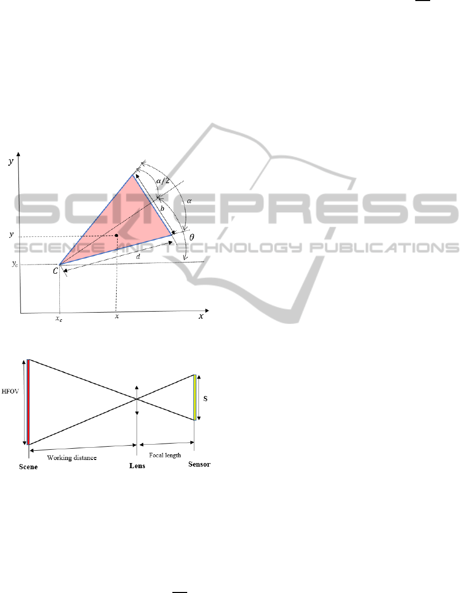
The parameters of the triangle, in Figure 1, are
calculated, given the camera intrinsic parameters and
the desired viewing resolution.
Figure 1: Field-of-view ∃
of sensor
in 2-D space.
Figure 2: Fundamental parameters of an imaging system.
Getting the FoV by a triangle allows describing the
area covered by each camera
, positioned at
,
and orientation ,with three linear
constraints:
cos.
sin.
y
(1)
.
.
y
2.
.
.
.
y
(2)
.
.
y
2.
.
.
.
y
(3)
Thus, each point, of the discretized monitoring
area can be observed by a camera
if the three
constraints (1), (2) and (3) are satisfied.
Theoretically, sensors can be placed anywhere in
the monitoring space since the sensor variables
,
and are continuous variables. Practically,
an approximation of the monitoring space by a two-
dimensional grid of points allows solving the
formulated optimization problem in discrete
representation .The distance between two grid points
in the and y directions is determined by the spatial
sampling frequencies:
,
:
1
⁄
;
1
⁄
(4)
Thus, cameras are constrained to be positioned only
at these discrete grid points, and coverage is
guaranteed relative to these grid points. The problem
becomes, then, a grid coverage problem.
So, given a discretized monitoring area and only
one type of camera, our problem is to find an
assignment of sensors to the grid of points such that
every point is covered by at least one sensor. Once
we defined the problem, visibility and environment
models, we solve it by defining the fitness function
and constraints as follows. Firstly, the fitness
function is to find the minimum number of cameras
to maximize the coverage.
,
,
(5)
Subject to
,
,
,
,θ
,
,
1
,1
(6)
,
,
1
1
, 1
1
(7)
Equation (6) guarantee that each grid point of the
monitoring space is covered by at least one camera
and equation (7) to ensure that only one camera can
be placed on each grid point.
In the case of different types of cameras such as
cameras with different working distances which
means different resolutions and optics (i.e., focal
ICINCO2014-11thInternationalConferenceonInformaticsinControl,AutomationandRobotics
254
lengths), the camera placement problem is similar to
the problem treated above. In this case, the goal is to
find the arrangement and the number of cameras
with different FoV parameters that minimize the
total cost while ensuring coverage. This optimization
problem is formulated as follows:
,
,,
(8)
Subject to
,
,,
,
,
,
,
1
(9)
Where is the total number of cameras and
is
the individual cost of each camera.
To insure that at each grid point only one camera
can be placed, we add the constraint below:
,
,,
1
,
1
,1
(10)
Where the binary variable
,
,
define whether
there is a camera in a grid point (,) . It is defined as
,
,
1Ifacameraispositionedatgrid
point
,
withorientation
0Otherwise
(11)
We define a binary variable to refer to the
points viewed by the different cameras in the 2-D
space.
,
,θ
,
,
1Ifacamerapositionedat
gridpoint
i
,j
with
orientationθcovergrid
point
i
,j
0Otherwise
(12)
3.2 PTZ Camera
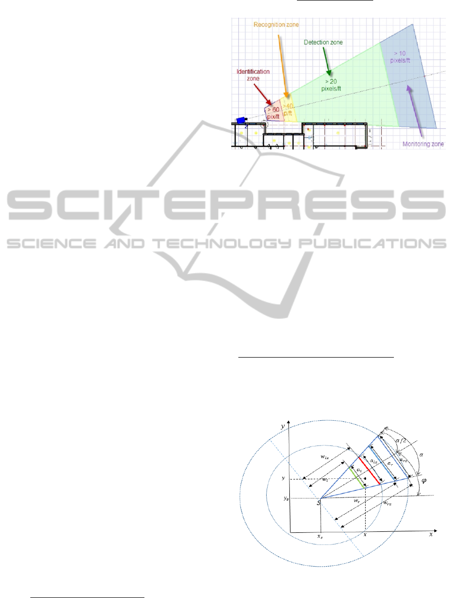
Our surface-projected PTZ camera model is shown
in figure 3. Based on the resolution requirements we
have modelled the PTZ camera .We have modelled
identification ,recognition and monitoring
visualization zones considering the resolution
needed for each task, which is used to calculate each
working distance for each visualization zone using
equations(13,14).
__
_
13
_
∗_
_
14
Figure 3: Surface-projected PTZ camera model based
resolution requirement.
The Figure. 4 represents the camera field of view
projected to the ground. The point (
,
)
corresponds to the camera position in the ground, the
working distances
,
corresponds to the
identification and recognition resolution respectively
and
,
corresponds to the identification and
recognition resolution respectively after zoom effect
and the orientation with respect to the axis,is
the FoV vertex angle.it is assumed that the PTZ
camera has 360° the extended field of view due to
motion.
To ensure that each grid point is identified which
ensure automatically the recognition task, it is
necessary to satisfy the two constraints:
.
.y
.
.y
(15)
.
.
y
0
(16)
Figure 4: Surface-projected PTZ camera model based
resolution requirement.
With this information, we compute the
OptimalCameraPlacementbasedResolutionRequirementsforSurveillanceApplications
255
assignment of cameras to grid points such that every
point is covered by at least one camera and the
coverage is maximized.
The objective function is to find the minimum
number of sensors to maximize the coverage given a
PTZ camera model, as
,
,
(17)
Subject to
,
,
,
,φ
,
,
1
,1
(18)
,
,
1
1
(19)
Equations (18) ensure that each grid point of the
monitoring space is identified by at least one camera
and equation (19) to ensure that camera has to be
located on a grid point. and only one camera can be
placed on each grid point.
Where the binary variable
1
,
1
,φ
represents
whether there is a PTZ camera in a point (,) . It is
defined as:
,
,
1Ifacameraispositionedatgrid
point
,
withorientation
0Otherwise
(20)
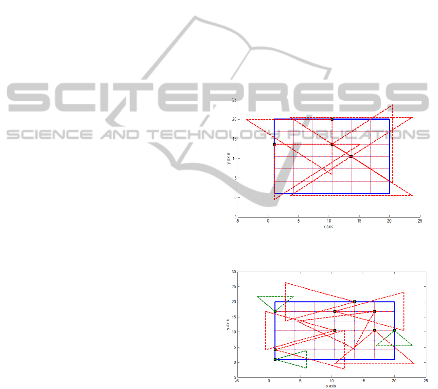
4 RESULTS
We show some results obtained using binary integer
programming algorithm in 2-D case.
We considered the case of one type of cameras
Figure 5. Then, two types of cameras Figure 6 where
a cost of 120 $ was assigned for the camera with the
larger FoV while only 80 $ was assigned for the
camera with the smaller FoV.
After we took in consideration the case of
presence of obstacles and essential zone which is
denoted as a critical and important zone which need
more attention at the time of monitoring operation
using two type of cameras Figure 7, Figure 9.
In all figures, bold blue lines represent the
borders of the area to be covered while the light
lines represent the area grid. The grid nodes to be
covered are the intersections points of these later
lines. The static camera’s FoV are represented by
triangles with dotted red lines in the case of only
type of cameras ,in the case of two types ,the second
type represented by a green dotted lines .The PTZ
cameras’ FOV are presented by a red triangles
showing the different working distances for the
different resolution requirements and the extended
FOV due to motion by a circler blue lines .The green
small squares represent the optimal position of the
cameras to be deployed for the placement ,the
obstacles is represented by a bold blue polygonal
and the essential zone by black rectangle .
4.1 Static Camera
In these subsection we took the four cases: one type
of cameras, different types of cameras, presence of
obstacles and the case of presence of essential zones.
Figure 5: Optimal placement of static cameras. (1 type of
camera,
10,
6,
6,
8,90°).
Figure 6: Optimal placement of static cameras. (2 type of
camera,
10,
4,
6,
6,
8,60°).
ICINCO2014-11thInternationalConferenceonInformaticsinControl,AutomationandRobotics
256
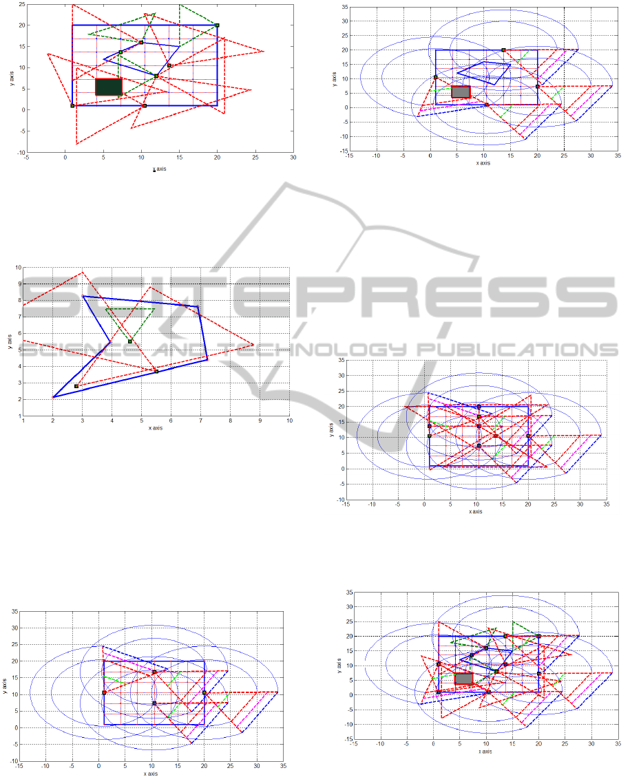
Figure 7: Optimal placement of static cameras
considering the presence of obstacle and essential zone. (2
type of camera,
10,
4,
6,
6,
8,60°).
Figure 8: Optimal placement of static cameras for complex
shape of monitoring area (2 type of camera,
10,
4,
6,
6,
8,60°).
4.2 PTZ Camera
For the simulation of a static cameras, we considered
the same monitoring area dimensions for figure 9
without with presence of obstacles and essential
zones, and in figure 10 we considered them.
Figure 9: Optimal placement of PTZ cameras. (
4,
6,
8,
10,
6,
6,
8,60°).
Figure 10: Optimal placement of PTZ cameras
considering the presence of obstacle and essential zone..
(
4,
6,
8,
10,
6,
6,
8,60°).
4.3 Static and PTZ Camera
For the simulation of mixtures of static and PTZ
cameras, we considered the same monitoring area
dimensions with and without presence of obstacles
and essential zones.
Figure 11: Optimal placement of static and PTZ cameras.
(
4,
6,
8,
10,
6,
6,
8,60°).
Figure 12: Optimal placement of static and PTZ cameras
with presence obstacles and essential zones. (
4,
6,
8,
10,
6,
6,
8,60°).
OptimalCameraPlacementbasedResolutionRequirementsforSurveillanceApplications
257

5 CONCLUSION
We have formulated an optimization problem on
camera placement based on a mixture of static and
PTZ cameras, where a minimum number of them are
spread out to provide a maximized coverage of the
monitoring area. The use of a combination of static
and PTZ cameras demonstrate functional to outlook
such as reduction in costs and information
processing. This is, because the PTZ camera can
monitor larger areas with every snapshot due to its
resolution capacity and extended FOV due to
motion.
Several interesting issues arise when one applies
our algorithm to a real situation. For instance, fixed
cameras are not able to recognize and identify
objects, because their resolution is limited, but they
are capable of detecting moving objects and this
result can be used to select the best PTZ camera
within the network to identify and recognize the
moving object
REFERENCES
E. Dunn, G. Olague, and E. Lutton. (2006). Parisian
Camera Placement for Vision Metrology,. Pattern
Recognition Letters, 27, 1209–1219.
E. Horster and R. Lienhart. (2006). Approximating
Optimal Visual Sensor Placement. IEEE International
Conference on Multimedia and Expo, 1257–1260.
J. Urrutia. (2000). Art Gallery and Illumination Problems.
in Handbook of Computational Geometry, 973–1027.
J. Wangand and N. Zhong. (2006). Efficient Point
Coverage in Wireless Sensor Networks. Journal of
Combinatorial Optimization, 11, 291– 304.
K. Chakrabarty, H. Qi, and E. Cho. (2002). Grid Coverage
for Surveillanceand Target Location in Distributed
Sensor Networks. Computers, IEEE Transactions, 51,
1448–1453.
Morsly, Y ; Aouf, N ; Djouadi, M.S and Richardson, M. t.
(2012). Particle swarm optimization inspired
probability algorithm for optimal camera network
placemen. IEEE Sens .J, 12, 1402–1412.
R. Lienhart and E. Horster. (2006). On the Optimal
Placement of MultipleVisual Sensor. in 4 th ACM
International Workshop on Video Surveillanceand
Sensor Networks, 111–120.
S. Chen and Y. Li . (2004). Automatic Sensor Placement
for Model-Based Robot Vision. Systems, Man and
Cybernetics IEEE Trans Syst, 33, 393–408.
S. S. Dhillon and K. Chakrabarty. (2003). Sensor
Placement for Effective Coverage
andSurveillanceinDistributedSensor Networks.
Wireless Communications and Networking WCNC-
IEEE,, 3, 1609–1614.
S. Thrun. (2002). Learning Occupancy Grids with
Forward Sensor Models. Autonomous Robots, 15,
111–127.
U. Murat and S. Sclaroff. (2006). Automated Camera
Layout to SatisfyTask-Specific and Floor Plan-
Specific Coverage Requirements. Computer Vision
and Image Understanding, 103, 156–169.
X. Chen and J. Davis. ( 2000). Camera Placement
Considering Occlusion for Robust Motion Capture.
Stanford University, Tech. Rep. CS-TR-2000-07.
ICINCO2014-11thInternationalConferenceonInformaticsinControl,AutomationandRobotics
258
