
Automated Segmentation of Folk Songs
Using Artificial Neural Networks
Andreas Neocleous
1,2
, Nicolai Petkov
2
and Christos N. Schizas
1
1
Department of Computer Science, University of Cyprus, 1 University Avenue, 2109 Nicosia, Cyprus
2
Johann Bernoulli Institute for Mathematics and Computer Science, University of Groningen, Groningen, The Netherlands
Keywords: Audio Thumbnailing, Singal Processing, Computational Intelligence.
Abstract: Two different systems are introduced, that perform automated audio annotation and segmentation of Cypriot
folk songs into meaningful musical information. The first system consists of three artificial neural networks
(ANNs) using timbre low-level features. The output of the three networks is classifying an unknown song as
“monophonic” or “polyphonic”. The second system employs one ANN using the same feature set. This
system takes as input a polyphonic song and it identifies the boundaries of the instrumental and vocal parts.
For the classification of the “monophonic – polyphonic”, a precision of 0.88 and a recall of 0.78 has been
achieved. For the classification of the “vocal – instrumental” a precision of 0.85 and recall of 0.83 has been
achieved. From the obtained results we concluded that the timbre low-level features were able to capture the
characteristics of the audio signals. Also, that the specific ANN structures were suitable for the specific
classification problem and outperformed classical statistical methods.
1 INTRODUCTION
The automatic annotation of a musical piece is an
important subject in the field of computational
musicology. The annotation of a musical piece
indicates interesting and important musical events.
Such events include the start and the end positions of
a note, the start and the end positions of a part in
which a singing voice is present, the repetitions of a
melody and others. This procedure is often called
audio thumb-nailing.
The main melody of a song is usually located
where a singing voice is present. The knowledge of
the position of a song that contains the main melody
can give insights in the structure of the song and it is
a starting point for further analysis and study. It is
also desirable to detect the part in a song where only
instruments are performing and no vocal singing is
present. This can be considered a classification task
of two classes. One class is the “vocal” where a
singing voice is performing and the other is the
“instrumental” where only instruments are
performing. Several methods that tend to solve
similar classification problems have been proposed
in the past by Lu et al (Lu, Zhang, Li, 2003),
Scheirer and Slaney (Scheirer and Slaney, 1997),
Fuhrmann et al (Fuhrmann, Herrera and Serra, 2009)
and Vembu and Baumann (Vembu and Baumann,
2005). Panagiotakis and Tziritas (Panagiotakis and
Tziritas 2004) propose a speech/music discriminator
based on the Root Mean Square (RMS) and the zero
crossing rates (ZCR). For the classification they
employ a set of rules such as void interval
frequencies between consecutive frames,
information gathered by the product between RMS
and ZCR, the probability of no zero crossings etc.
Another common approach is the extraction of
features from a training set that was previously
annotated with the desired classes and the
application of standard machine learning techniques.
In the work of Pfeiffer et al, (Pfeiffer, Fischer and
Effelsberg, 1996) perceptual features such as
loudness or pitch were taken into account in their
experiments. They claim that these features play a
semantic role for the performance of their
classifications and the audio content analysis.
Experiments with additional features rather than
using only the RMS and the ZCR were also
introduced by Scheirer et al and Slaney (Scheirer
and Slaney, 1997).
The latest publication and the most relevant to our
work, is found in literature by Bonjyotsna and
Bhuyan (Bonjyotsna and Bhuyan, 2014). They
144
Neocleous A., Petkov N. and N. Schizas C..
Automated Segmentation of Folk Songs Using Artificial Neural Networks.
DOI: 10.5220/0005049101440151
In Proceedings of the International Conference on Neural Computation Theory and Applications (NCTA-2014), pages 144-151
ISBN: 978-989-758-054-3
Copyright
c
2014 SCITEPRESS (Science and Technology Publications, Lda.)

suggest as main feature the Mel-Frequency Cepstral
Coefficients (MFCC) for the classification of
vocal/instrumental parts applied in the
MUSCONTENT database. Three machine learning
techniques were used for the classification: Gaussian
Mixture Model (GMM), Artificial Neural Network
(ANN) with Feed Forward Backpropagation
algorithm and Learning Vector Quantization (LVQ).
From their results, they claim that LVQ yields the
higher accuracy in the classification. More precisely,
they report 77% classification accuracy for the
ANNs, 77.6% for the LVQ and 60.24% for the
GMM. In our work, we included additional low-
level features and we achieved higher accuracy by
modeling our data with ANN.
In this paper, we introduce a two-stage approach
for (a) the classification of an unknown song into
“monophonic” or “polyphonic” and (b) the
segmentation of a polyphonic song into positions of
interest. Such positions include the boundaries of a
part in a song that only instruments are performing
and no vocal singing is present. We used low-level
timbre features and we built trained artificial neural
networks that are able to discriminate and predict
with high accuracy the unknown songs as
“monophonic” or “polyphonic” and polyphonic
music as “vocal” or “instrumental”.
The main contribution of our work is the use of
ANNs and their application in audio thumb-nailing.
This use has numerous advantages in wide range of
applications (Benediktsson, J., et. al., 1990). The
ability of the adaptation of complex nonlinear
relationships between variables arises from the
imitation of the biological function of the human
brain. Disadvantages include the greater time of
training, and the empirical nature of model
development. The authors have demonstrated how
the disadvantages can be minimized in a wide area
of applications including medicine (Neocleous C.C.,
et. al. 2011).
While the interest of the MIR community on the
audio thumb-nailing focused in popular music, little
work has been done for folk music. Main differences
between popular music and folk music include the
western/non-western instrumentation as well as
fundamental rules in music theory. For instance, the
use of traditional instruments in folk music, create a
significantly different sound in comparison to the
popular music. One common feature of the folk
music is the monophonic performances. These can
be either using a musical instrument or only with
singing voice. Our contribution with a classification
system of a song into “monophonic” or
“polyphonic” is reported in this paper.
We compare our results with two other methods,
named Support Vector Machines and the statistical
Bayesian Classification.
2 METHODS
2.1 Overview
The database we used contains audio signals of 98
Cypriot folk songs. Each audio signal has been
extracted from original cd’s and it has been encoded
with a sampling frequency of 44100 Hz and 16 bit
amplitude. The sampling frequency of 44100 Hz and
the amplitude of 16 bit is the quality that is typically
used in the audio cd’s.
From this database, we isolated 24 songs for
creating a training set while the remaining 74 songs
were used for validation of our system. In the
training set, 17 monophonic songs and 7 polyphonic
songs were chosen. The monophonic songs were 6
vocal songs sung by male performers, 6 vocal songs
sung by female performers and 5 songs performed
with the traditional Cypriot instrument called
“pithkiavli”.
The main idea of our method is illustrated in
Figure 1. The first system takes as input an unknown
song and predicts if it is monophonic or polyphonic.
The second system takes a polyphonic song and
predicts the boundaries of parts of the song that only
instruments are performing (instrumental parts) and
parts in which a singing voice is present (vocal
parts).
Each audio signal was segmented into a sequence
of overlapping audio frames of length 2048 samples
(46 ms) overlapping by 512 samples (12 ms). For
each of these audio frames we extracted the
following audio features: Zero Crossing Rate,
Spectral Centroid, MFCC (13 coefficients). For the
first system the mean and the standard deviation
values of each feature are calculated and are used to
build three feed-forward ANNs. Each of them has 20
neurons in the hidden layer and was trained for 200
epochs. The ANNs were built using monophonic
songs for the first class and polyphonic songs for the
second class. The difference between the three
ANNs is that the instrument that is performing in the
monophonic songs is different for each network.
This system classifies an unknown song into the
class “monophonic” or “polyphonic”. Both systems
1 and 2 require audio frame segmentation and
feature extraction.
For the second system, the entire feature vectors
were used to build one ANN that predicts a value in
AutomatedSegmentationofFolkSongsUsingArtificialNeuralNetworks
145
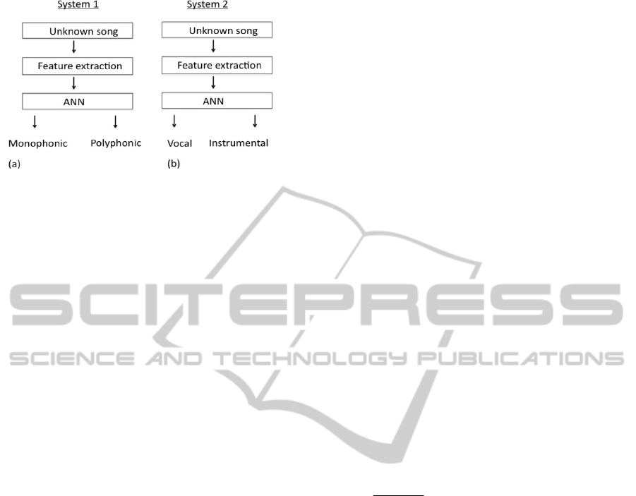
Figure 1: (a) System 1 takes as an input an unknown song
and classifies the song as “monophonic” or “polyphonic”.
(b) System 2 takes as an input a polyphonic song and
segments it into “vocal” and “instrumental” parts.
the range between 0 and 1 for every audio frame.
The output is then quantified with a threshold to the
binary values 0 or 1. The value 0 corresponds to a
frame from a purely instrumental part. The output is
1 if vocal singing is present in the frame. We use
this system to annotate the instrumental and the
vocal parts in a song.
2.2 Neural Network
Many different ANN structures had been proposed
and used by researchers in different fields. The most
common and widely used for classification,
generalization, and prediction is the commonly
known fully connected multilayer feed forward
structure (FCMLFF). Mathematically this is
represented by equation 1 as:
1
1
,1
1
][
,1
][][][
L
L
LL
n
j
L
LL
L
j
L
iL
L
iL
wyfy
(1)
where,
][L
iL
y
is the output value of each neuron
iL
of
layer L that has a total of
nL
neurons.
Typically, this function has a squashing
function form such as the logistic or the
hyperbolic tangent.
LL
W
,1
is the set of weights associating neurons in
layer L-1 to neurons in layer L.
Once the ANN is decided, an effective training
and tuning procedure needs to be implemented, so
that the network will achieve a useful capability for
doing the desired task, such as classification,
generalization, recognition etc. Many training
procedures had been proposed and are available for
implementation. The most widely used for feed
forward networks is the backpropagation algorithm
(Werbos, 1974). In this work, we implemented fully
connected feed-forward neural networks with
backpropagation learning.
2.3 Feature Selection
Twenty-four songs were selected to form a training
set to be used in the artificial neural network
classifier. The training set was chosen in such a way
that all the musical instruments that were of our
interest for classifying them were present. The
positions of the vocal parts and the instrumental
parts were manually annotated to the training data
and a set of low-level timbre features were extracted
for each class respectively. Specifically, the features
extracted were the Zero Crossing Rate, Spectral
Centroid, Spectral Spread and 13 coefficients of
MFCC, thus creating a feature set of 16 features in
total. We applied a statistical analysis to the features
and from the results we assume that this set of
features is considered to be suitable for solving the
particular classification problem.
2.3.1 Zero Crossing Rate
The feature Zero Crossing Rate (Benjamin 1986) is
a measure on how many times does the waveform
crosses the value of zero within a frame:
1
1
)](sgn[)1(sgn[
)1(2
1
N
n
nxnx
N
ZCR
(2)
Where:
)(nX
: is the discrete audio signal, n=1…N
sgn[.]: is a sign function.
The ZCR is a powerful feature for identifying
noisy signals. It is also used as a main feature for
fundamental frequency detection algorithms (Roads
1996).
2.3.2 Spectral Centroid
The feature Spectral Centroid it is the geometric
center of the distribution of the spectrum and is a
measure of the spectral tendency of a random
variable x. It is a useful feature for classification
problems such as instrument identification or the
separation of audio signals into speech/music. It is
defined as:
dxxxf )(
1
(3)
Where:
x: is a random variable
NCTA2014-InternationalConferenceonNeuralComputationTheoryandApplications
146

f(x): is the probability distribution of the random
variable x characterized by that distribution.
2.3.3 Spectral Spread
The feature Spectral Spread it is defined in eq. 4 and
it is essentially the standard deviation of the
spectrum. It describes how much energy is
distributed by the frequencies across the spectrum.
dxxfx )()(
2
(4)
2.3.4 Mel Frequency Cepstral Coefficients
(Mfcc)
The feature MFCC (Mermelstein 1976) describes
the timbre characteristics of an audio file within a
number of coefficients. Usually the number of the
coefficients taken into account is 13. The
computation of the MFCCs is as follow: first the
spectrum of a framed windowed excerpt audio signal
is computed using the Fast Fourier Transformation
(FFT). The result from the FFT is then mapped into
13 Mel bands using triangular overlapping windows.
The cosine transformation is applied to the logarithm
of each one of those Mel bands. The results of each
transformation for every band are considered to be
the MFCC coefficients. The mapping of the
spectrum from the linear scale to the Mel scale is
done in order to approximate the functionality of the
human auditory system where, in one of its
processes it separates the perceived sound into non-
linear frequency bands. The most popular formula
for converting the frequencies from hertz to Mel is
described below:
700
1log2595
10
f
mel
(5)
Where:
f: is the frequency in Hertz.
The mel scale has been proposed by Stevens et al
in 1937 (Stevens, Volkman and Newman, 1937) and
the name comes from the word melody. It is pointed
that the MFCC features are widely used in speech
processing and are considered to be a powerful
feature for describing timbre characteristics. They
carry most of the spectral information within 13
coefficients, in contrast with the row spectrum that
has at least 5000 frequency values. In Figure 2 we
present an example of the spectrogram of a
polyphonic song for an excerpt of 50 seconds. In this
case, there are three positions where only
instruments are performing, and two positions where
the singing voice is also performing together with
the instruments. The first parts of the instrumental
and the singing voice are annotated in the same
Figure, on the lower plot. It is rather obvious that the
distribution of the energy across the spectrum for the
two classes “vocal” and “instrumental” is different.
Figure 2: Spectrogram of a polyphonic song. The first 15
seconds in this figure are being performed with
instruments. The position from the 15
th
to 20
th
second is
performed with singing voice together with instruments. It
is shown that the distribution of the energy across
frequencies between the two positions “instrumental” and
“vocal” significantly differ.
Figure 3 shows the 13 coefficients of the MFCC
features for the same excerpt of the same song. It is
also clear that the MFCC in the instrumental part
have higher values with respect to the part of a
singing voice.
Figure 3: The 13 coefficients of MFFCs versus time. The
“instrumental” and the “vocal” parts are annotated
manually in the lower plot.
2.4 Statistical Analysis
In an attempt to visualize the data and to understand
AutomatedSegmentationofFolkSongsUsingArtificialNeuralNetworks
147
better the contribution of each feature to the
performance of the system, we applied statistical
methods and we report our results in this section. In
this analysis we are concerned to explore how
significant is the difference between the values of a
given feature for the two classes “instrumental” and
“vocal”. Our null hypothesis is that the median of
the data in class “instrumental” is equal with the
median of the data in class “vocal”.
Several methods exist for testing a statistical
hypothesis, such as z-test, t-test, Chi-squared test,
Wilcoxon signed-rank test and others. The t-test is
the most widely used method for testing significant
differences between two populations whose size is
less than 30 (Mankiewicz, R., 2004). It assumes that
the distribution of the two populations being
compared is normal. In our case, not all features we
used are following a normal distribution. More
precisely, the features Zero Crossing Rate, Spectral
Centroid and Spectral Spread did not follow a
normal distribution for any of the two classes. These
features were tested with the Wilcoxon signed-rank
test (Siegel, 1956). The 13 coefficients of the MFFC
were following a normal distribution. The normality
of each distribution was tested with a graphical
method and with the Kolmogorov-Smirnov test
(Stephens, 1974). For the graphical method we used
a normal probability plot. In order to get such plot,
first the histogram of the data is approximated with a
normal distribution.
In the normal probability plot, the probability
distribution follows a normal distribution and it is
plotted against the unknown distribution of the data.
If the data follow a normal distribution, the function
of the normal probability plot will be a straight line.
If the normal probability plot does not fit to a
straight line, it is an indication that the distribution
of the data does not follow a normal distribution. In
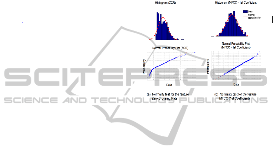
Figure 4 we present an example of this method for
the features (a) Zero Crossing Rate and (b) MFCC of
the first coefficient.
In Figure 4a the upper plot shows with blue color
the distribution of the feature ZCR and with red
color the normal approximation. From this plot it is
obvious that the normal distribution cannot model
the distribution of the data. This is also observable
from the normal probability plot in the lower plot. In
Figure 4b we present an example where the
distribution of the data of the feature MFCC can be
modeled with a normal distribution.
The Wilcoxon signed-rank test is a non-
parametric method for testing the significance of the
difference between two populations. This method
does not assume that the distribution of the
populations is normal. We used this method for
testing the features that did not have normal
distribution. For the 13 MFFC coefficients we used
the t-test. Both the t-test and the Wilcoxon signed-
rank test rejected the null hypothesis that the two
populations are not different for all the features we
used.
Figure 4: Normality test for the features (a) ZCR and (b)
MFCC. In the upper plot, the histogram of every feature is
plotted together with the approximation with a normal
distribution. Lower plot shows the normal probability
plots.
2.5 Classification into “Monophonic”
or “Polyphonic”
For the classification into the two classes
“monophonic” or “polyphonic” we built three ANN
using the mean and the standard deviation of each
feature. In total, 32 features were used to train the
ANNs. The first ANN is called “male vocal –
polyphonic” and is trained with 720 seconds of
monophonic male singing performances which form
the first class and 115 seconds of polyphonic music
which form the second class. The second ANN is
called “female vocal – polyphonic” and is trained
with 720 seconds of monophonic female singing
performances (1st class) and the same 115 seconds
of polyphonic music (2nd class). The third ANN is
called “pithkiavli – polyphonic” and is trained with
600 seconds of monophonic performances by the
instrument “pithkiavli” (1st class) and 115 seconds
of polyphonic music (2nd class). The output target
for the polyphonic music was set to 1 and the output
target for the class “female vocal”, “male vocal” and
“pithkiavli” was set to 0.
The classification is done with the following
procedure: an unknown song is represented
numerically by a vector of 32 that is fed to the three
NCTA2014-InternationalConferenceonNeuralComputationTheoryandApplications
148
ANN “male vocal - polyphonic”, “female vocal -
polyphonic” and “pithkiavli - polyphonic”. We
quantize the outputs of the models to 0 or 1 by using
a threshold of 0.5. We classified a song as
“monophonic” if the binary output of at least two
models is 0; otherwise the song is classified as
“polyphonic”.
2.6 Classification into “Vocal” or
“Instrumental”
The fourth ANN was built using all feature vectors
that were extracted for all audio frames. The output
target was added to the database after a manual
segmentation of the training set into the “vocal” and
“instrumental” positions. For every audio frame of a
song the ANN gives a prediction value in the range
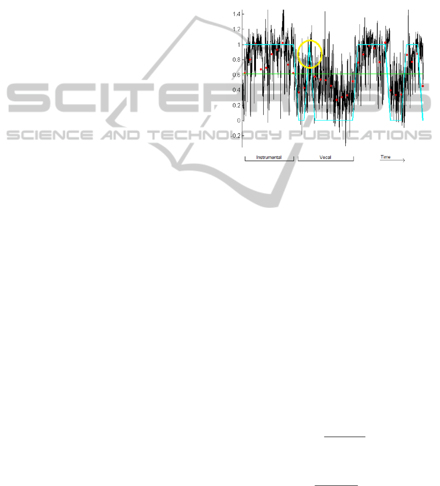
0 or 1. One example of the output of the ANN is
shown in Figure 5 with continuous black line. The
vocal parts and the instrumental parts are annotated
manually. Even though in this example it is shown
that most of the output values correspond to the
correct class (if we set a threshold), some of the
frames are misclassified.
In order to solve the misclassification problem, we
introduced a set of rules and we used dynamic
programming for correcting the possible
misclassifications. In a first step we divide the frame
sequence in groups of 100 frames each and we
compute their vector mean as shown with red dots in
Figure 5. These values are then converted into
binary vales by using an appropriate threshold. The
threshold is calculated as the mean of the mean
values and is shown with green line in the same
figure. In this example the threshold is 0.6. The
mean values that fall above the threshold are
classified as “instrumental” while the values that fall
below the threshold are classified as “vocal”.
Further processing was needed in order to correct
additional misclassifications. One example of a
misclassified sample is encircled in figure 5. In this
example, the encircled output value exceeds the
threshold and the system wrongly classifies that
position as instrumental. For solving such
misclassification problems, we introduced the
following rule:
Each sample of the quantized vector is tested with
the classes that belong to the frames around it. To
consider a classification of a sample as true, the
class of the previous frame has to be the same with
the class of the following two frames. Regardless on
what the classification of the testing frame is, after
we apply this rule, the classification may change.
In order to illustrate an example, in Figure 5 we
present a frame that was wrongly classified as
instrumental while the annotation of this frame is to
be vocal. This frame is encircled with yellow colour
and in this example it is the testing frame. The
previous frame and the two frames after the testing
frame belong to the class “vocal” while the testing
frame belong to the class “instrumental”. After we
apply the rule described above, the class of the
testing frame turns from “instrumental” to “vocal”.
Figure 5: Black continuous line shows the output of the
ANN for a chunk of 30 seconds of a polyphonic song. Red
dots show the mean values for groups of 100 frames each.
Blue continuous line shows the binary quantization of the
mean values with respect to the threshold. Yellow circle
shows an example of a misclassified value.
3 EVALUATION AND RESULTS
The validation set contained 74 songs of a total
duration of 230 minutes. 46 songs were monophonic
and the remaining 28 were polyphonic. For the
classification of the “monophonic – polyphonic”, we
call a “false positive” prediction when a song is
annotated as “monophonic” and the prediction of the
system is “polyphonic”. We present our results in
terms of precision and recall. ANNs achieved a
precision of 0.88 and recall of 0.78. SVMs gave
precision of 0.85 and recall of 0.81 and Bayesian
Statistics precision of 0.71 and recall of 0.69.
The precision is defined as:
F
PTP
TP
precision
(6)
The recall is defined as:
FN
T
P
TP
recall
(7)
AutomatedSegmentationofFolkSongsUsingArtificialNeuralNetworks
149

For the classification of the “vocal – instrumental”
we call a false positive if a part of the signal was
annotated as “vocal” but the prediction of the system
was “instrumental”. Figure 6 shows an example on
how we define the terms false positive, false
negative and true positive for the specific
classification problem. The audio signal is plotted
with black continuous line. The red vertical lines
indicate the limits in the audio signal where only
instruments are performing, while the green vertical
lines indicate an example of the limits where a
prediction was done from our system. We call false
positive the duration of the signal that the ground
truth is annotated as “vocal” and the prediction was
“instrumental”. ANNs achieved a precision of 0.85
and recall of 0.83. SVMs gave precision of 0.86 and
recall of 0.82 and Bayesian Statistics precision of
0.76 and recall of 0.72.
Figure 6: The interpretation of the terms “false positive”,
“True positive” and “False negative”.
Where:
TP: True positive
FP: False positive
FN: False negative
4 CONCLUSIONS
We described a method for automatic annotation of
Cypriot folk music into “polyphonic” or
“monophonic” music. In the validation procedure,
the audio signal is segmented into audio frames of
46 ms. A set of low level features are being
extracted from each such audio frame and given to
the input layer of the neural network. In the output
layer, a value between 0 and 1 is extracted. This
value is used for the classification using a threshold.
For polyphonic music we presented an automatic
annotation into instrumental or singing parts. The
system identifies these positions by classifying each
audio frame into instrumental or vocal. This is done
automatically, while there is no need for any
external assistance or guidance.
From our experiments we observed that timbre
low-level features are suitable to capture the
characteristics of each class. The advantage of our
system is the use of ANNs and standard timbre low-
level features. We consider ANNs a very powerful
technique for classification problems. They have the
ability to imitate the biological function of the
human brain. Thus, they are able to efficiently
identify patterns and correlations in the feature
space. Our method does not need any perceptual
features and it uses the row values of the features
without any pre-processing such as feature
normalization. The selected features are state of the
art for audio analysis and classification.
The ANNs and the SVMs had similar results. In
comparison with the statistical Bayesian
classification the ANNs and the SVMs performed
better. We present a precision of 0.78 and recall of
0.88 for the first system and a precision of 0.85 and
recall of 0.83 for the second system. The results are
not yet finalised but represent the basis on our future
research will be based. Improvements of the results
reported in this paper could be achieved by
introducing additional features such as mid-level
features. Principal component analysis could also be
applied to the feature set for dimensionality
reduction. These problems are currently under study
and the results will be reported in the near future.
ACKNOWLEDGEMENTS
This work is supported by the research grant
Ανθρωπιστικες/Ανθρω/0311(ΒΕ)/19 funder by the
Cyprus Research Promotion Foundation.
REFERENCES
Bonjyotsna A., Bhuyan M., 2014. Performance
Comparison of Neural Networks and GMM for
Vocal/Nonvocal segmentation for Singer
Identification. International Journal of Engineering
and Technology (IJET), Vol. 6, No 2.
Benediktsson J., Swain P, and Ersoy, O., 1990. Neural
Network Approaches Versus Statistical Methods in
Classification of Multisource Remote Sensing Data.
IEEE Transactions on Geoscience and Remote
Sensing, Vol. 28, No 4.
Benjamin, K., 1986. Spectral analysis and discrimination
by zero-crossings. In Proceedings of the IEEE, pp.
1477–1493.
NCTA2014-InternationalConferenceonNeuralComputationTheoryandApplications
150

Fuhrmann, F, Herrera, P, Serra, X., 2009. Detecting Solo
Phrases in Music using Spectral and Pitch-related
Descriptors. Journal of New Music Research, 2009,
pp. 343–356.
Lu, L, Zhang, H, J, Li, S, Z., 2003. Content-based audio
classification and segmentation by using support
vector machines. In Multimedia Systems.
Mankiewicz, R., 2004. The Story of Mathematics.
Princeton University Press, p. 158.
Mermelstein, P., 1976. Distance measures for speech
recognition, psychological and instrumental. Pattern
Recognition and Artificial Intelligence, pp. 374–388.
Muller, M, Grosche, P, Wiering, F., 2009. Robust
segmentation and annotation of folk song recordings.
International Society for Music Information Retrieval
(ISMIR), pp. 735–740.
Neocleous C.C., Nikolaides K.H., Neokleous K.C.,
Schizas C.N. 2011, Artificial neural networks to
investigate the significance of PAPP-A and b-hCG for
the prediction of chromosomal abnormalities. IJCNN -
International Joint Conference on Neural Networks,
San Jose, USA.
Panagiotakis, C, Tziritas, G., 2004. A Speech/Music
Discriminator Based on RMS and Zero-Crossings. In
IEEE Transactions on Multimedia.
Pfeiffer, S, Fischer, S, Effelsberg, W., 1996. Automatic
Audio Content Analysis. In Proceedings of the fourth
ACM international conference on Multimedia, pp. 21-
30.
Roads, C., 1996. The Computer Music Tutorial. MIT
Press.
Scheirer, E, Slaney, M., 1997. Construction and evaluation
of a robust multi feature speech/music discriminator.
In IEEE International Conference On Acoustics,
Speech, And Signal Processing, pp. 1331–1334.
Siegel, S., 1956. Non-parametric statistics for the
behavioral sciences. New York: McGraw-Hill, pp. 75–
83.
Stephens, M, A., 1974. EDF Statistics for Goodness of Fit
and Some Comparisons. Journal of the American
Statistical Association (American Statistical
Association), pp. 730–737.
Stevens, S, S, Volkman J, Newman, E, B., 1937. A scale
for the measurement of the psychological magnitude
pitch. Journal of the Acoustical Society of America,
pp. 185–190.
Vembu, S, Baumann, S., 2005. Separation of vocals from
polyphonic audio recordings. International Society for
Music Information Retrieval (ISMIR), pp. 337–334.
Werbos P., 1974. Beyond Regression: New Tools for
Prediction and Analysis in the Behavioural Sciences.
Ph.D. dissertation Applied Mathematics, Harvard
University.
AutomatedSegmentationofFolkSongsUsingArtificialNeuralNetworks
151
