Optimization Strategies for Tuning the Parameters of Radial Basis

Functions Network Models

Gancho Vachkov

, Nikolinka Christova

and Magdalena Valova

School of Engineering and Physics, The University of the South Pacific (USP), Laucala Campus, Suva, Fiji

Department of automation of Industry, University of Chemical Technology and Metallurgy, Sofia, Bulgaria

Keywords: Radial Basis Function Networks, RBF Models, Parameter Tuning, Optimization Strategies, Particle Swarm

Optimization, Supervised Learning.

Abstract: In this paper the problem of tuning the parameters of the RBF networks by using optimization methods is

investigated. Two modifications of the classical RBFN, called Reduced and Simplified RBFN are

introduced and analysed in the paper. They have a smaller number of parameters. Three optimization

strategies that perform one or two steps for tuning the parameters of the RBFN models are explained and

investigated in the paper. They use the particle swarm optimization algorithm with constraints. The one-step

Strategy 3 is a simultaneous optimization of all three groups of parameters, namely the Centers, Widths and

the Weights of the RBFN. This strategy is used in the paper for performance evaluation of the Reduced and

Simplified RBFN models. A test 2-dimensional example with high nonlinearity is used to create different

RBFN models with different number of RBFs. It is shown that the Simplified RBFN models can achieve

almost the same modelling accuracy as the Reduced RBFN models. This makes the Simplified RBFN

models a preferable choice as a structure of the RBFN model.

1 INTRODUCTION

Radial Basis Function (RBF) Networks have been

widely used for a long time as a power tool in

modeling and simulation, because they are proven to

be universal approximators of nonlinear input-output

relationships with any complexity (Poggio, Girosi,

1990; Park, Sandberg, 1993). In fact, the RBF

Network (RBFN) is a composite multi-input, single

output model, consisting of a predetermined number

of N RBFs, each of them performing the role of a

local model (Pedrycz, Park, Oh, 2008). Then the

aggregation of all the local models in the form of a

weighted sum of their output produces the nonlinear

output of the RBFN.

There are some important features that make the

RBF networks diferent from the classical feed

forward networks, such as the well known

multilayer perceptron (MLP), often called back-

propagation neural network (Poggio, Girosi, 1990);

Zhang, Zhang, Lok, Lyu, 2007). The biggest difference

is that the RBFN are heterogeneous in parameters.

In fact they have three different groups of

parameters, which normally require the use of

different learning algorithms. This makes the total

learning process of the RBFN more complex,

because it is usually done as a sequence of several

learning steps. This obviously affects the accuracy

of the produced model.

In this paper we investigate in details the internal

structure of the RBFN and propose two

modifications of the classical RBFN, called Reduced

and Simplified RBFN. They have smaller number of

tuning parameters, which makes the learning faster.

As an universal optimization procedure for tuning all

three groups of parameters we use in the paper a

modified version of the classical Particle Swarm

Optimization (PSO) (Eberhart, Kennedy, 1995) with

specific constraints for each group of parameters.

This constrained version produces more plasusible

solutions of parameters with real physical meaning.

The rest of the paper is organized as follows.

Section 2 summarizes the basics of the classical

RBFN model and Section 3 introduces the Reduced

and Simplified RBFN wilth smaller number of

parameters. Section 4 expalinjs three different

optimization strategies for creating RBFN models

that use a modification of the PSO algorithm with

constraints. In Section 5 one-stap optimization

strategy is used for tuning the parameters of the

443

Vachkov G., Christova N. and Valova M..

Optimization Strategies for Tuning the Parameters of Radial Basis Functions Network Models.

DOI: 10.5220/0005051104430450

In Proceedings of the 4th International Conference on Simulation and Modeling Methodologies, Technologies and Applications (SIMULTECH-2014),

pages 443-450

ISBN: 978-989-758-038-3

 2014 SCITEPRESS (Science and Technology Publications, Lda.)

Reduced and Simplified RBFN models. Finally,

Section 6 concludes the paper.

2 THE CLASSICAL RBF

NETWORK MODEL

Our aim is to create a model of a real process

(system) with K inputs and one output by using a

collection of M available experiments (input-output

pairs) in the form:

{( , ),...,( , ),...,( , )}

ii M M

yy yXXX

(1)

Here

[, ,..., ]

xxX

is the vector of all K inputs

and

is the respective measured output from the

process.

The modelled output, calculated by the RBF

network is as follows:

(,)

yf XP

(2)

Here

[ , ,..., ]

ppP is the vector of all L

parameters included in the RBFN.

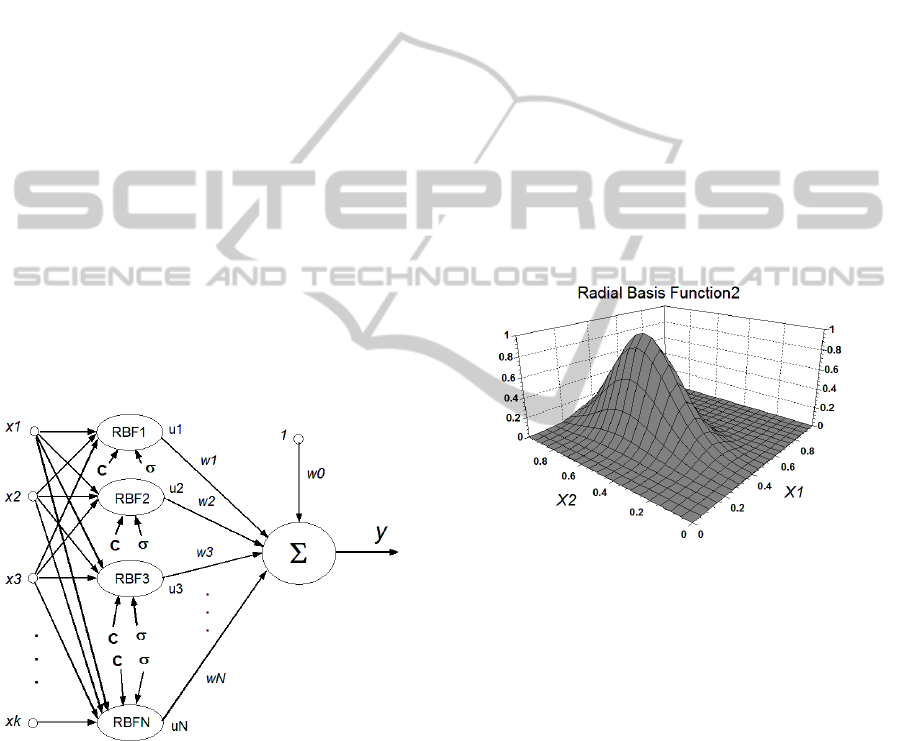
The classical RBFN has a three layer structure,

namely input layer, hidden layer and output layer as

shown in Fig. 1.

Figure 1: Structure of the Classical Radial Basis Function

Network with K inputs and N RBFs.

Then the modelled output from the RBFN with fixed

number of N Radial Basis Functions will be:

mii

wwu







(3)

Here

, 1, 2,...,

ui N

are the outputs of each RBF

based on its K inputs

and

, 0,1, 2,...,

wi N



are the weights associated with

the RBFs, including the offset weight

w as seen in

the figure.

Each RBF is determined in the K-dimensional

space by two groups (vectors) of parameters, namely

the center (location)

[ , ,..., ]

cc c



and the

width (spread)

[ , ,..., ]







. Then the output

u of each RBF is calculated as:

exp[ ( ) /(2 )]

exp [( ) /(2 )] [0,1]

jj j

uxc





 



 









(4)

Figure 2 shows a 3-dimensional plot of one RBF

calculated by (4) with K=2 inputs and the following

vectors for the center and width in the input space:

[0.4, 0.6]; [0.10,0.20]



C σ

Figure 2: Example of a RBF with K=2 Inputs, center

location at [0.4, 0.6] and two different widths: [0.10, 0.20].

It is now clear that all parameters form the following

3 groups in the parameter vector P, namely: Centers,

Widths and Weights, as follows:

[, ,..., ]

pp pPCσ W



(5)

Then, for a RBFN with K inputs and N RBFs, the

total number L of the parameters to be tuned will be:

(1)2( ) 1LNK NK N N K N



   

(6)

It is obvious that the number of all L parameters will

rapidly grow with increasing the complexity of the

RBFN model, i.e. the number of RBFs and the

number of inputs. This possesses a challenge to the

selected learning algorithm.

, ,...,

SIMULTECH2014-4thInternationalConferenceonSimulationandModelingMethodologies,Technologiesand

Applications

444

3 TWO MODIFICATIONS OF

THE RBF NETWORK MODEL

In order to reduce the total number L of parameters

that have to be tuned (optimized), we propose and

use in this paper two modifications of the classical

RBFN model from (3) and (4) shown in Fig. 1.

3.1 The Reduced RBF Network

The reduction of the number of parameters here is

achieved by assuming that the RBF has a scalar

width



instead of a K-dimensional vector width

[ , ,..., ]





σ as in (4). Then the calculation

of the output for each RBF is performed according

to the Euclidean distance between the input vector X

and the center C of the RBF, as follows:

exp ( ) (2 ) [0,1]

uxc







  







(7)

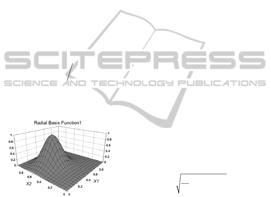
An example of one RBF with a scalar width

0.15





and center

[0.4,0.6]C

is shown in Fig. 3.

It is easy to notice the difference in the shape with

the RBF in Fig. 2.

Figure 3: Example of a RBF with K=2 Inputs, center

location at [0.4, 0.6] and a single width of 0.15.

Now the total number L of the parameters in the

proposed Reduced RBFN is calculated as:

(1) 21LNK N N NK N  

(8)

3.2 The Simplified RBF Network

This is a further step in reducing the number L of all

parameters of the RBF network. Here an assumption

of one common width



for all N RBFs is made.

This means that the calculation of each RBF is

performed by the same equation (7), as in the

Reduced RBFN, but with one common width



for

all RBFs. Now the total number L of the parameters

in the proposed Simplified RBFN will be:

1( 1) 2LNK N NK N



 

(9)

The idea of creating a model by the Simplified RBF

Network is that that all N RBFs will be located (in

general) at different locations (centers) in the K-

dimensional input space, but will have one common

width Sigma. Here it could be expected that a large

number of RBFs will be needed (compared with the

case of Reduced RBFN) in order to achieve the same

or similar model accuracy. However this speculation

needs to be proven experimentally.

4 OPTIMIZATION STRATEGIES

FOR PARAMETER TUNING OF

THE RBF NETWORK MODEL

Further on we assume that the collection (1) of M

input-output pairs of experiments is available and

the structure of the RBFN is fixed prior to the

learning process. This means that the number N of

the RBFs is fixed and the structure of the RBFN

(Classical, Reduced or Simplified) is decided.

The next step is to tune in off-line mode all L

parameters (5) of the RBFN model so that to

minimize a preliminary formulated performance

index. Since this is a typical supervised learning

problem, the objective here is to minimize the total

prediction error (RMSE) by the RBFN model, as

follows:

()min

iim

RMSE y y







(10)

The problem of tuning (training) the parameters of

the RBF network is a typical (off-line or online)

supervised learning problem, which can be solved

by a nonlinear optimization method. This problem

has been investigated by many authors for a long

time by using different algorithms (Musavi, Ahmed,

Chan, Faris, Hummels, 1992

; Yousef, 2005). The

work presented in this paper is considered as our

viewpoint and approach to solving the problem.

As mentioned in Section 2, there are 3 different

groups of parameters in the RBFN model, namely

centers, widths and weights, according to the

notations in (3). The objective of minimizing the

RMSE in (10) can be achieved by use of different

learning and optimization strategies. They are

summarized briefly as follows:

OptimizationStrategiesforTuningtheParametersofRadialBasisFunctionsNetworkModels

445

Strategy 1. This is a two-step strategy. First the

vector P of all parameters from (5) is divided into

two groups: Group1, consisting of the centers C and

widths



and Group2, consisting of the weights W.

Then the first step of the Strategy 1 performs

unsupervised learning algorithm (such as the C-

means clustering algorithm) to find the locations of

the centers in the input space. Then an approximate

estimation of the widths is performed as a post-

processing heuristic procedure. The second step is

an optimization procedure of the Group 3 parameters

- the weights, according to the criterion in (10).

Strategy 2. This is another two step strategy. The

first step performs the same unsupervised clustering

algorithm, as in Strategy 1, but this time for finding

the location of the centers only. Then the second

step performs optimization on the remaining two

groups or parameters: the widths and the weights.

Strategy 3. This is a one-step optimization strategy

that is performed on all three groups of parameters

in (5), namely the centers, widths and weights.

It is expected that the Strategy 3 has the potential

to be the best one, since here all 3 groups of

parameters are being optimized simultaneously.

However the actual practical results will strongly

depend on the quality of the algorithm for

multidimensional optimization, as well as on the

proper definition of the boundaries for all three

groups of parameters.

The sequel of the paper is focused mainly on the

use of Strategy 3 for tuning the parameters of the

Reduced and the Simplified RBFN models and on

the analysis of their performance. The widely

popular Particle Swarm Optimization (PSO) (Poli,

Kennedy, Blackwell, 2007) is used as a basic

optimization algorithm with some modifications for

Strategy 3.

4.1 Basics of the Standard Particle

Swarm Optimization (PSO)

Algorithm.

The PSO belongs to the group of the multi-agent

optimization algorithms. It uses a heuristics that

mimics the behaviour of flocks of flying birds

(particles) in their collective search for a food. The

main concept of this algorithm is that a single bird

has no enough power to find the best solution, but in

cooperation and exchanging information with other

birds in the neighbourhood the swarm is likely to

find the best (global) solution. The swarm consists

of a predetermined number n of particles (birds) that

perform a limited cooperation at each iteration of the

search.

At each iteration the PSO algorithm changes the

velocity (step)

v and the position

x of the particles

1, 2,...,in



according to the following equations:

(0, ) ( )

ii ii

iii













vvU px

Upx

xxv

(11)

Here

(0, )



is a vector of random numbers

uniformly distributed in the range

[0, ].



At each

iteration one number is randomly generated for each

particle.



is a component-wise multiplication;

p is the coordinate (location) of the personal best

success of the i-th particle;

is the coordinate (location) of the global best

success so far and g is the index of this particle;



is the so called “inertia weight”. The introduction

of this parameter in the main equation (11) is the

most popular modification of the classical PSO

algorithm. In fact the inertia weight parameter

controls the power of the particles during the search.

In order to make a proper ratio and plausible balance

between the two stages: exploration and exploitation

in the search, this coefficient is initially set to a

relatively high value ( 0.9, 1.0 or higher) and then is

gradually decreased by each iteration to another,

lower value (e.g. 0.3). This represents the physical

meaning of birds being gradually exhausted (tired)

during search. Most often a predefined linear

decreasing function is used to change the inertia

weight.

Normally the PSO algorithm stops when a given

criterion, such as maximal fitness or minimal error is

met. Since it cannot be always guaranteed, in the

practical implementations of the PSO additional

safety measure, namely a predetermined number of

iterations is used to terminate the algorithm.

4.2 Modified Version of the PSO

Algorithm with Constraints

It is important to note that the classical version of

the PSO does not include constraints (boundaries) on

the search in the input space. This is because of the

general assumption that birds are free to explore the

whole unlimited space so that eventually they can

find the global optimum. It is clear that the width of

the exploration area and the exploration success of

the birds will depend on their current “power”,

SIMULTECH2014-4thInternationalConferenceonSimulationandModelingMethodologies,Technologiesand

Applications

446

which is defined by the amount of the velocity (step)

at the current iteration, according to (11).

In almost all practical engineering problems it is

mandatory to impose certain constraints (limits) to

the parameters of the input space

[, ,..., ]

order to produce an optimal solution with a clear

physical meaning that can be practically realized.

Therefore we have made here a slight modification

in the original version of the PSO algorithm with

inertia weight in order to consider both constraints

(minimum and maximum) on the input parameters, as

follows:

1min 2min min

[, ,..., ]

xx x

1max 2max max

[, ,..., ]

xx x

(12)

The idea here is very simple, namely the respective

input parameter from

[, ,..., ]

which has

violated the input space is moved back to its

boundary value from (11), as follows:

min min

()

jj jj

Fx x THENx x and

max max

()

jj jj

Fx x THENx x

. (13)

In such way, at the next iteration a new velocity

(step) from (11) will be generated that has different

amount and direction in the input space. As a result

the particle is likely to escape from being trapped in

the area beyond the boundary. This of course, could

take sometimes not one, but a few iterations.

The next subsection displays some results from the

performance of the constraint version of the PSO.

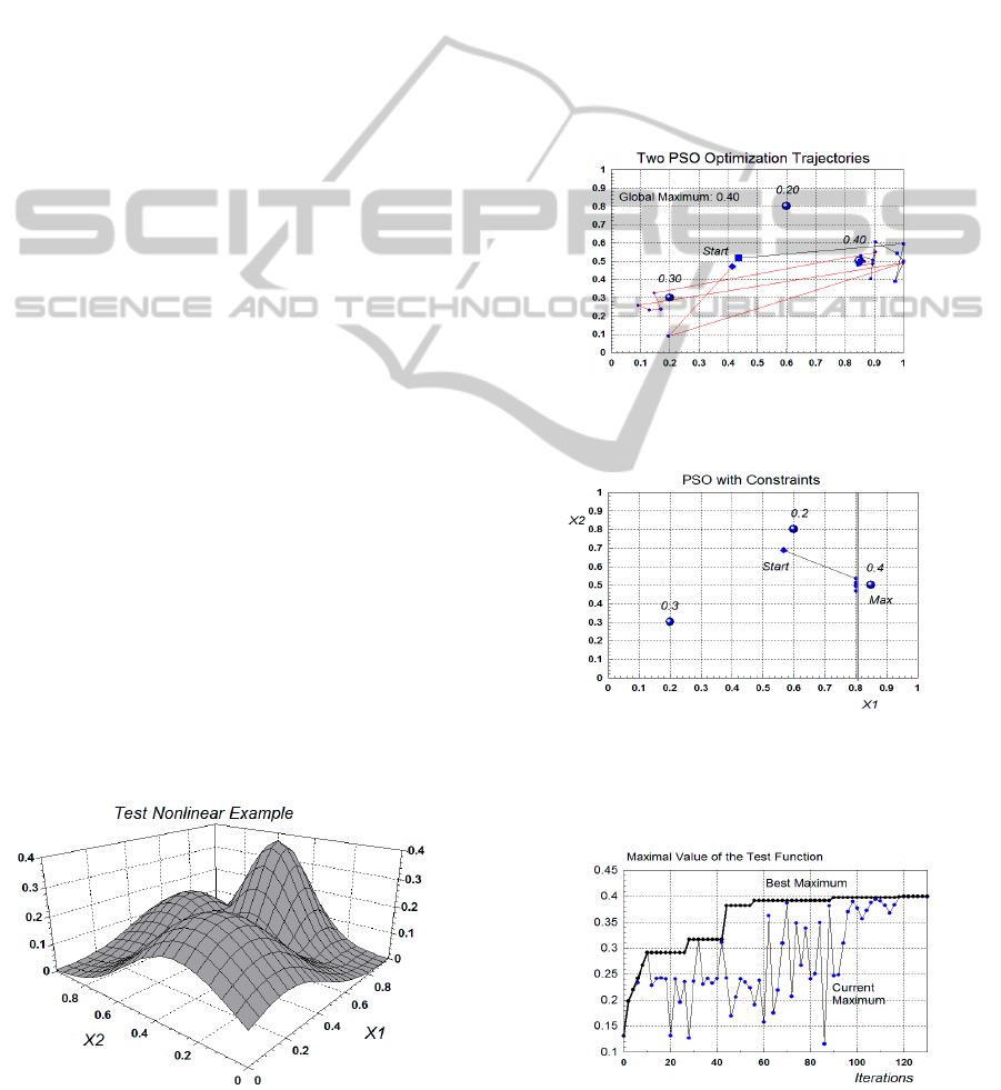
4.3 PSO Performance Evaluation on a

Test Nonlinear Example

A highly nonlinear test example with 2 inputs and

one output is shown in Fig. 4. It was specially

generated in order to evaluate the performance of the

PSO algorithm with constraints.

Figure 4: The test nonlinear example used for performance

evaluation of the PSO algorithm with constraints.

The example is synthetic and constructed by

using 3 RBFs with special overlapping, as seen from

the figure. As a result the response surface (the

output) has 3 maximums (two local and one global)

and the value of the global maximum is 0.4.

The normal range of the input parameters is [0,1]

and the results from two runs of the PSO algorithm

with constraints is shown in Fig. 5. The algorithm

succeeded to find the global maximum of 0.4 after

respective corrections in the trajectories at the

boundary of

1max

1.0x



according to (13).

The next Fig. 6 depicts a case of constrained

optimization, where the PSO algorithm succeeded to

find a conditional maximum at the “wall” of the

constraint.

Figure 5: Two different trajectories, produced by two runs

of the PSO algorithm with constraints at the boundary 1.0

for finding the global maximum of 0.4.

Figure 6: A conditional maximum found by the PSO with

constraints at the boundary 0.8 for the input x1.

The convergence curve for the PSO algorithm, based

on the test example is shown in Fig. 7.

Figure 7: Convergence curve that shows the performance

of the PSO algorithm on the test example.

OptimizationStrategiesforTuningtheParametersofRadialBasisFunctionsNetworkModels

447

5 EXPERIMENTAL RESULTS

FROM OPTIMIZATION OF

REDUCED AND SIMPLIFIED

RBFN MODELS

5.1 The Experimental Setup

The main goal in this section is to compare the

performance of the Reduced RBFN model (Section

3.1) with the Simplified RBFN model (Section 3.2).

As seen from (6), (8) and (9), both models have a

smaller number of parameters, compared with the

parameters in the classical RBFN from Section 2.

The comparison was performed on the same

synthetic test nonlinear example from Fig. 4 that was

used in Section 4 to evaluate the performance of the

PSO algorithm with constraints. The difference is

that now our aim is to create two models, namely

Reduced RBFN and Simplified RBFN of the same

2-dimensional process from Fig. 4 by using a given

set of M input-output experimental data.

For solving this supervised learning problem, we

use the one-step Strategy 3, explained in Section 4

for simultaneous tuning in off-line mode the all 3

groups of parameters. Here the PSO algorithm with

constraints from Section 4.2 was used.

It is seen from (8) and (9) that the Simplified

RBFN model has smaller number of parameters than

the Reduced RBFN model. In fact, if the selected

number of RBFs is N = 8, the Reduced RBFN will

have L=33 parameters, while the Simplified RBFN

will need only L=26 parameters for tuning.

We would like to see whether the Simplified

RBFN is able to produce a model with a similar

(without significant deterioration) performance to

that one of the Reduced RBFN model. A positive

answer to this question would be beneficial for the

Simplified RBFN models.

We use in this paper a set of M=441 uniformly

distributed experimental data in the two-dimensional

space [X1, X2] produced by scanning.

Due to the random nature of the PSO algorithm,

it cannot be expected that one single run will

necessarily produce the absolute global optimum.

Therefore we have performed several (six in this

paper) runs of the algorithm for the same pre-

selected number N of RBFs. At each run the

parameters of the PSO algorithm were slightly

varied. Then the mean value of the RMSE in (10)

from all six runs was assumed as a final

representative value of the error for this number N.

All the experiments were performed separately

for the Reduced and Simplified RBFN with the

following numbers of RBFs: N = 3,4,5,6 and 8. The

constraints imposed to each of the 3 groups of

parameters in (5) were as follows:

- The group of Centers:

min max

0, 1cc

;

- The group of Widths:

min max

0.02, 0.7





;

- The group of Weights:

min max

1, 1ww 

The tuning parameters of the PSO algorithm with

constraints were varied during the multiple runs in

following ranges:

- Number of particles:

15 40n



;

- Number of iterations:

12000 15000

MAX

IT

;

- Acceleration Coefficients:

,[1.8,2.1]





;

- Inertia Weight parameter



: linearly decreasing

from initial values

[0.9,1.2]





at the first

iteration, to

[0.3,0.4]





at the last iteration.

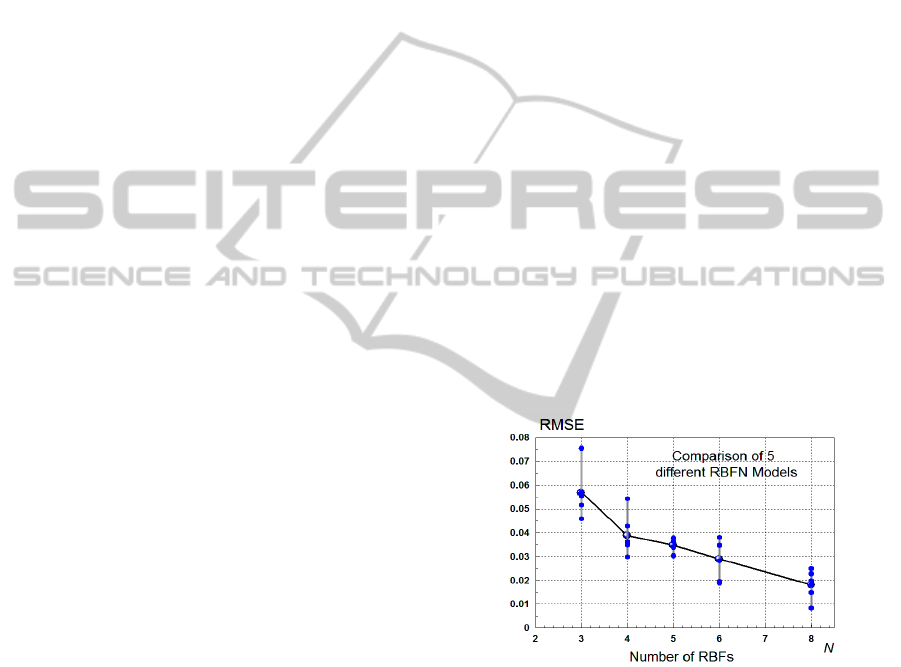
5.2 Experiments with the Reduced

RBFN Model

The main results from these experiments are

displayed in a graphical way in Fig. 8. It is seen

from the figure that the accuracy of the models is

steadily improved with increasing the number of the

RBFs, which is a logical and understandable.

Figure 8: Experimental results obtained from Reduced

RBFN models with different number of RBFs.

For one intermediate RBFN model with N=4 and

respective RMSE=0.0428 the response surface (the

outputs of the model) is shown in Fig. 9. A visual

comparison of the shape of this surface with the

surface for the original process in Fig. 4 reveals

relatively large difference, i.e. the model is not yet

suitable for a good prediction.

The best obtained model is with N=8 RBFs and

has RMSE = 0.00826. Its response surface is

displayed in Fig. 10. It is easy to notice that this

surface practically coincides in shape with the

surface produced by the original process from Fig. 4.

SIMULTECH2014-4thInternationalConferenceonSimulationandModelingMethodologies,Technologiesand

Applications

448

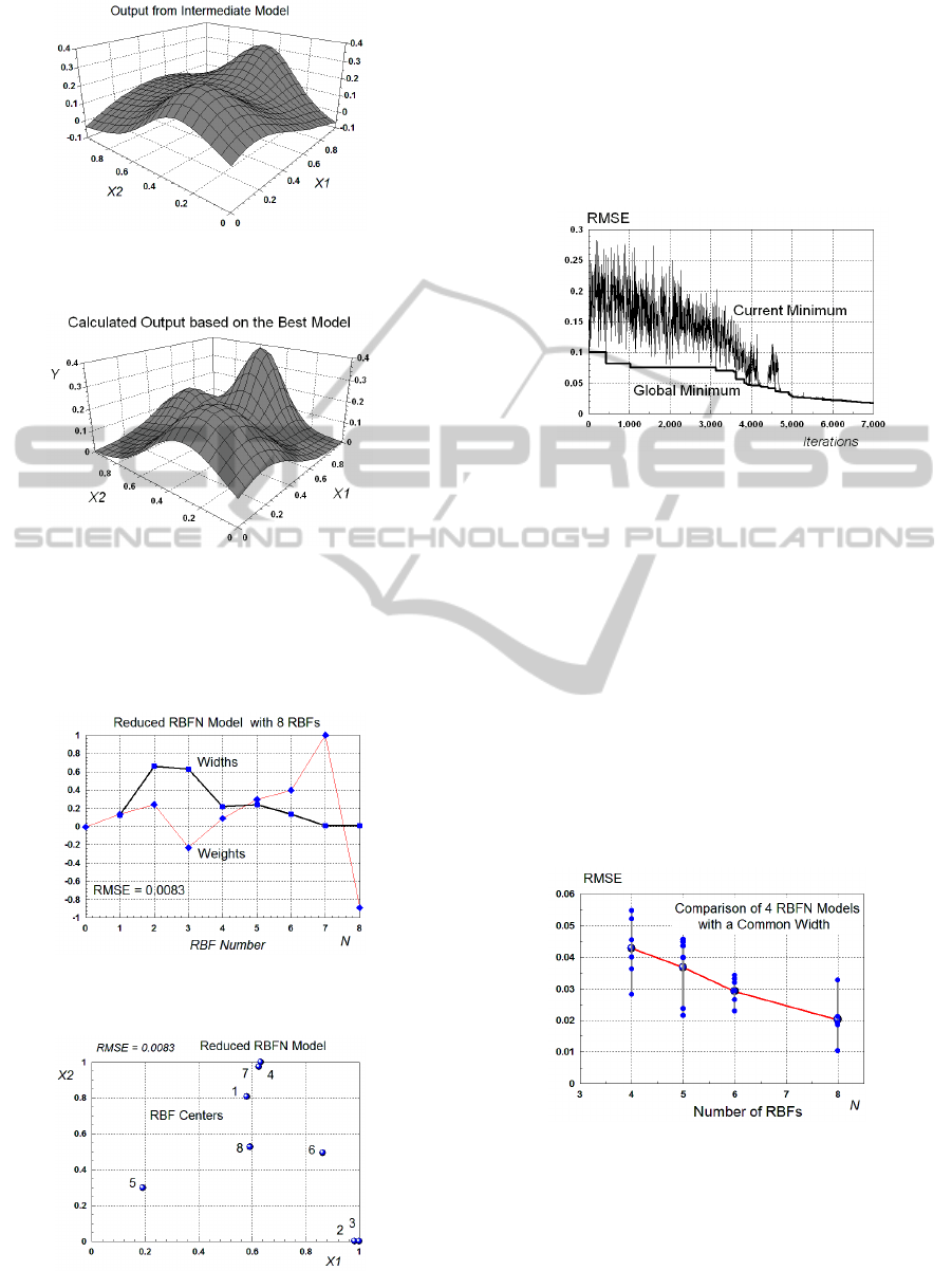
Figure 9: Response surface from the intermediate Reduced

RBFN model with N = 4 RBFs and RMSE = 0.0428.

Figure 10: Response surface from the best Reduced RBFN

model with N = 8 RBFs and RMSE = 0.0083.

The values of all parameters (Centers, Widths and

Weights) for the best model from Fig. 10, are

displayed in Fig. 11 and Fig. 12.

Figure 11: The values of the Widths and Weights for the

best Reduced RBFN model with N=8 RBFs.

Figure 12: Locations of all 8 Centers of the best produced

Type2 RBFN model with N=8 and RMSE = 0.0083.

From Fig. 12 it is seen that some of the centers

are placed at the boundaries of the input space and

some others have insignificant widths (closer to

zero). This shows that there is a redundancy in the

number of the parameters or in the number of the

RBFs.

The convergence curve for the best Reduced

RBFN model is shown in Fig. 15.

Figure 13: Convergence curve for the PSO algorithm with

constraints in the case of the best model with N=8 RBFs.

5.3 Experiments with the Simplified

RBFN Model

The same structure of the experiments for the

Reduced RBFN was used for producing the results

for the Simplified RBFN models. The results with

the respective RMSE of all the Simplified RBFN

models are shown in Fig. 14 and the parameters of

the best model with N=8 and RMSE=0.0104 are

shown in Fig. 15 and Fig. 16. Note that the

Simplified RBFN model has one common width

Sigma for all RBFs, with an optimal value of

0.1494.

Figure 14: Experimental results obtained from the

Simplified RBFN models with different number of RBFs.

The trend in Fig. 14 of a gradual decrease of the

RMSE with increasing the number of the RBFs is

similar to the trend shown in Fig. 8 for the Reduced

RBFN models. Also, a comparison of the values for

the mean RMSE in both figures reveals that there are

OptimizationStrategiesforTuningtheParametersofRadialBasisFunctionsNetworkModels

449

similar. Therefore a conclusion could be made that

the Simplified RBFN model is able to achieve

almost the same accuracy as the Reduced RBFN

model, but with smaller number of parameters,

namely L=26 versus L=33.

Figure 15: The values of the Weights for the best

Simplified RBFN model with N=8 RBFs and one common

Width.

Figure 16: Locations of all 8 Centers of the best

Simplified RBFN model with N=8 and RMSE = 0.0104.

It is seen from Fig. 15 and Fig. 16 that RBF1 (shown

as Center 1 in Fig. 16) is inactive, because its weight

is zero (as seen from Fig. 15). This is another case of

redundancy in the parameters (or in the number of

RBFs) of the model.

6 CONCLUSIONS

The investigations in this paper were focused on the

performance analysis of the RBFN models with two

slightly different structures, namely the Reduced

RBFN and Simplified RBFN models.

One of the three optimization strategies

explained in this paper is the one-step Strategy3,

which optimizes simultaneously all three groups of

parameters, namely the Centers of the RBFs, their

Widths and the Weights. A modified version of the

PSO algorithm with constraints was used for tuning

the parameters of both Reduced and Simplified

RBFN models on a test nonlinear example with

different number of the RBFs.

The Simplified RBFN model has the smallest

number of parameters, because it uses one common

width for all RBFs, unlike the Reduced RBFN

model that uses different widths for the RBFs.

The simulation results have shown that despite

the smaller number of parameters, the Simplified

RBFN models are able to achieve almost the same

accuracy, as the Reduced RBFN models. Therefore

the Simplified RBFN could be the preferable choice

for creating RBFN models.

The further research is focused on solving

another optimization problem such as the optimal

selection of the RBF units used in creating the

RBFN models.

ACKNOWLEDGEMENTS

This paper has been produced with the financial

assistance of the European Social Fund, project

number BG051PO001-3.3.06-0014. The authors are

responsible for the content of this material, which

under no circumstances can be considered as an

official position of the European Union and of the

Ministry of Education and Science of Bulgaria.

REFERENCES

Poggio, T., Girosi, F., 1990. Networks for approximation

and learning. Proceedings of the IEEE, 78, 1481-1497.

Musavi, M., Ahmed, W., Chan, K., Faris, K., Hummels,

D., 1992. On the training of radial basis function

classifiers. Neural Networks, 5, 595–603.

Park, J., Sandberg, I.W., 1993. Approximation and radial-

basis-function networks. Neural Computation, 5, 305–

316.

Eberhart, R.C., Kennedy, J., 1995. Particle swarm

optimization. In: Proc. of IEEE Int. Conf. on Neural

Network, Perth, Australia (1995) 1942–1948.

Yousef, R., 2005. Training radial basis function networks

using reduced sets as center points. International

Journal of Information Technology, Vol. 2, pp. 21.

Zhang, J.-R., Zhang, J., Lok, T., Lyu, M., 2007. A hybrid

particle swarm optimization, back-propagation

algorithm for feed forward neural network training.

Applied Mathematics and Computation 185, 1026–

1037.

Poli, R., Kennedy, J., Blackwell, T., 2007. Particle swarm

optimization. An overview. Swarm Intelligence 1, 33–

57.

Pedrycz, W., Park, H.S., Oh, S.K., 2008. A Granular-

Oriented Development of Functional Radial Basis

Function Neural Networks. Neurocomputing, 72, 420–435.

SIMULTECH2014-4thInternationalConferenceonSimulationandModelingMethodologies,Technologiesand

Applications

450