
Self-calibration of Large Scale Camera Networks
Patrik Goorts, Steven Maesen, Yunjun Liu, Maarten Dumont, Philippe Bekaert and Gauthier Lafruit
Hasselt University - tUL - iMinds, Expertise Centre for Digital Media
Wetenschapspark 2, 3590 Diepenbeek, Belgium
Keywords:
Calibration, Feature Matching, Multicamera Matches, Outlier Filtering.
Abstract:
In this paper, we present a method to calibrate large scale camera networks for multi-camera computer vi-
sion applications in sport scenes. The calibration process determines precise camera parameters, both within
each camera (focal length, principal point, etc) and inbetween the cameras (their relative position and orien-
tation). To this end, we first extract candidate image correspondences over adjacent cameras, without using
any calibration object, solely relying on existing feature matching computer vision algorithms applied on the
input video streams. We then pairwise propagate these camera feature matches over all adjacent cameras us-
ing a chained, confident-based voting mechanism and a selection relying on the general displacement across
the images. Experiments show that this removes a large amount of outliers before using existing calibration
toolboxes dedicated to small scale camera networks, that would otherwise fail to work properly in finding
the correct camera parameters over large scale camera networks. We succesfully validate our method on real
soccer scenes.
1 INTRODUCTION
In the current multimedia landscape, entertainment
delivery in the living room is more important than
ever. Users expect more and more impressive con-
tent to stay entertained. Therefore, new technologies
have been developed, such as 3D television, graphical
effects in movies, interactive television, and more.
We will focus on a single use case of novelcontent
creation, i.e. computer vision applications in soccer
scenes. In this application, a large number of cam-
eras are placed around the field, creating a large scale
camera network. These cameras are then used to gen-
erate novel virtual viewpoints (Goorts et al., 2014) or
create tracking information of the players on the field.
To make such applications possible, the cameras
should be geometrically calibrated, i.e. their intrin-
sic properties (focal length, principal point, etc) as
well as their relative position and orientation (extrin-
sic parameters) should be estimated (Hartley and Zis-
serman, 2003, page 178). For small scale camera net-
works many approaches exist for intrinsic and extrin-
sic calibration under controlled conditions. Most of
them work by moving calibration objects in front of
the cameras, such as checker board patterns (Zhang,
2000) and laser lights (Svoboda et al., 2005), pro-
viding corresponding feature points in the respective
camera views for extracting intrinsics and extrinsics,
as explained in section 3.
In this paper, we will present a system to calibrate
a large scale camera network placed around the pitch
of a sport scene, here demonstrated in a soccer game.
We demonstrate our method using eight cameras, but
any arbitrary number of cameras can be used. Be-
cause access to the pitch is restricted and the scale is
very large, we will present a self-calibration system
that does not use any calibration objects, such as the
methods of (Ohta et al., 2007) and (Grau et al., 2005).
The main contribution of this paper is the gen-
eration of reliable multicamera image correspon-
dences with a minimum of outliers, for efficient self-
calibration. This avoids a calibration recording pro-
cess, reducing cost and effort. These correspondences
are used in calibration toolboxes intended for small
scale camera networks. We use the toolbox of (Svo-
boda et al., 2005) for estimating the intrinsic and ex-
trinsic parameters.
Correspondence determination and matching is
typically used between two images. Features are de-
tected out of each image separately, and their statisti-
cal descriptors are pairwise matched between two im-
ages. This will, however, not suffice for our applica-
tion, where feature matches between multiple images
are required. Therefore, we present a system to gener-
ate multicamera matches by propagating the matches
between successive pairs of images.
107
Goorts P., Maesen S., Liu Y., Dumont M., Bekaert P. and Lafruit G..
Self-calibration of Large Scale Camera Networks.
DOI: 10.5220/0005057201070116
In Proceedings of the 11th International Conference on Signal Processing and Multimedia Applications (SIGMAP-2014), pages 107-116
ISBN: 978-989-758-046-8
Copyright
c
2014 SCITEPRESS (Science and Technology Publications, Lda.)
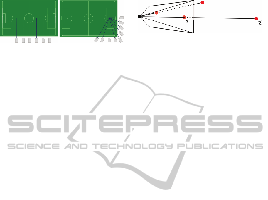
(a) (b)
Figure 1: Two possible camera arrangements for soccer
scenes. Both arrangements have different properties. (a)
In the linear arrangement, all cameras are placed on a line
next to the long side of the pitch and have the same look-at
angle. (b) In the curved arrangement, all cameras are placed
around a corner of the pitch and point to a spot in the scene.
These multicamera matches might, however, be
unreliable. Therefore, we also present a filtering ap-
proach that is specifically tailored to cameras placed
next to each other, without a relative rotation around
their optical axes. Even large scale, curved cam-
era pathways can be properly handled by following a
piecewise linear approach over each triple of adjacent
camera views. We remove many outliers that would
not be removed with existing calibration tools, effec-
tively improving the calibration quality.
There are a number of existing camera calibration
methods available for outdoor sport scenes that do not
use calibration objects. Most of these methods use the
lines of the soccer area to determine camera locations
(Farin et al., 2003; Farin et al., 2005; Li and Luo,
2004; Yu et al., 2009; Hayet et al., 2005; Thomas,
2007). They are therefore only applicable if the scene
is a soccer pitch, where the lines are planar and visible
over all camera views. This is, however, not always
the case. The pitch is seldom a plane and cameras
with a small field of view do not always have lines in
their image stream. We therefore propose a solution
without this planar line assumption, which makes our
large-scale calibration solution more robust and more
widely applicable, with good self-calibration perfor-
mances (i.e. not requiring any specific calibration ob-
ject).
The rest of the paper is structured as follows. Sec-
tion 2 describes the used camera setup, with its geo-
metrical properties recorded into camera matrices, as
explained in section 3. Section 4 discusses the gen-
eration of the multicamera correspondences and their
propagation over adjacent cameras. Finally, section
5 describes our multicamera filtering approach to fur-
ther dismiss apparant outliers.
2 CAMERA SETUP
We do not present a camera calibration method for
Figure 2: The projective camera model. A camera center
and an image plane is defined. The image is formed by con-
necting a line between the camera center and the 3D point.
The intersection between this line and the image plane de-
fines the position of the projection for that 3D point.
all possible camera setups. Instead, we will present a
camera method for a large scale camera network, with
the following properties.
We considered two possible arrangements for the
cameras: a linear arrangement and a curved ar-
rangement with piecewise linear properties over large
scales. These camera topologies are shown in Fig-
ure 1. In both arrangements, the cameras are placed
around the pitch at a certain height to allow an
overview of the scene. Both the curved and linear ar-
rangement use cameras with a fixed location and ori-
entation. Some overlap between the camera images is
required to allow feature matching. Overlap between
every camera is, however, not required.
Our method requires that the cameras are synchro-
nized at shutter level, i.e. all cameras take an image at
the exact same time stamp. To provide this, we use
a pulse generator that periodically transmits a trigger-
ing pulse to all cameras at the same time.
3 REPRESENTATION OF
CAMERA PARAMETERS
In this section, we giveanoverviewof projectivecam-
eras and their matrix representations, commonly used
in computer vision applications.
A simple pinhole camera maps each 3D scene
voxel to a corresponding 2D image pixel, through
projection along the light rays traversing the pinhole.
Any real camera with a lens and finite aperture fol-
lows this basic voxel-to-pixel mapping principle and
can hence conveniently be modeled by an equivalent
pinhole camera. We will assume that all cameras fol-
low the pinhole projective camera model, as defined
by (Hartley and Zisserman, 2003, page 6) and shown
in Figure 2.
This projective process can be mathematically
represented in matrix notation as follows. Consider
a 3D point χ, represented in homogeneous coordi-
nates. In essence, homogeneous coordinates repre-
sent a point χ = [X,Y,Z]
T
, using four coordinates χ =
[WX,WY,WZ,W]
T
withW 6= 0 or χ = [X,Y, Z,1]
T
. A
SIGMAP2014-InternationalConferenceonSignalProcessingandMultimediaApplications
108

Figure 3: Intinsic and extrinsic camera matrices explained.
The point χ and the camera center are defined in an arbitrary
coordinate system. Multiplying by M will transfer the cam-
era to the origin of the coordinate system, and χ will have
the same relative position. Multiplying by K will project χ
to the image plane.
projective camera now transforms this 3D point χ in
a homogeneous 2D point x = [x,y,1]
T
using a projec-
tion matrix P:
x = Pχ ⇔
x
y
1
= P
X
Y
Z
1
Here, the projection matrix P can be split up in
two sets of components: intrinsic and extrinsic pa-
rameters, represented by the intrinsic matrix K and
the extrinsic matrix M, with P = KM.
The intrinsic camera parameters represent the re-
lation between a 2D pixel location and its correspond-
ing 3D ray, presuming the camera is placed at the ori-
gin, and the image plane is parallel to the XY plane
at Z = f, where f is the focal distance. The line per-
pendicular to the image plane and passing through the
center of projection is called the principal axis, while
the point where the principal axis intersects the image
plane is called the principal point. The principal point
can be represented as a 2D point (p
x
, p
y
) on the image
plane. The 3× 3 matrix K is then given by:
K =
f 0 p
x
0 f p
y
0 0 1
Using x = Kχ for a camera placed at the origin
with an image plane Z = f, x is the image coordinate
on the image plane with principal point (p
x
, p
y
).
However, the camera is seldomly placed at the
origin, especially if multiple cameras are involved.
Therefore, the 3×4 extrinsic matrix M is used, which
transforms 3D voxels to a new location and orienta-
tion, so that the intrinsic matrix K is applicable (Hart-
ley and Zisserman, 2003, page 155). The matrix M
consists of a rotation and a translation, as shown in
Figure 3, and has the following form:
M =
R −R
˜
C
where R is a 3 × 3 rotation matrix and
˜
C is the
camera location in non-homogeneous coordinates.
In essence, M will translate and rotate the world
such that the camera is placed at the world origin,
where K will then project the 3D voxels to the image
plane, resulting in the final, projected image.
Using this camera model, the calibration process
then consists of determining these projection matri-
ces, when only the images of the cameras are given.
To this end, we acquire image correspondences using
feature matching, use them to generate the projection
matrices, and then finally split these projection matri-
ces into their intrinsic and extrinsic components using
the QR decomposition (Hartley and Zisserman, 2003,
page 579), which exploits the triangular shape of ma-
trix K.
4 DETERMINATION OF 2D
IMAGE CORRESPONDENCES
We determine image point correspondences by us-
ing a feature detector on all synchronously captured
images individually, followed by all possible combi-
nations of pairwaise matching. To increase robust-
ness, feature matching between each pair of images is
done in two directions, i.e. find the matches from im-
age 1 to image 2, and cross-check with the matches
from image 2 to image 1. A number of pairwise fea-
ture detectors were tested (Doshi et al., 2010), includ-
ing the SIFT (Lowe, 2004) and SURF (Bay et al.,
2006), where SIFT proved to provide the most reli-
able matches on our dataset.
The configuration of the cameras determine the
exact approach for finding matches. If the cameras
are far away from each other, only groups of three se-
quent cameras are considered to find matches. This
avoids extreme outliers resulting from matches over
images that contain a very different part of the scene.
If the cameras are placed in an arc, one camera can
have a view angle perpendicular to the view angle of
another camera. This will make matching of features
on players unreliable and is therefore avoided by us-
ing only three successive cameras.
If the cameras are close to one another and there
is a large overlap between all cameras, matches be-
tween all pairs of images are searched for. We will
select matches between all cameras using a consen-
sus based searching approach.
For a multicamera match to qualify for use in cali-
bration, it has to contain features of at least three cam-
eras and the matching in each image pair has to be
Self-calibrationofLargeScaleCameraNetworks
109

Figure 4: The graph used in our example. Nodes A - G are features detected in a set of images, each of which is taken by a
different camera at the same moment. The red edges show mismatches between features, the black correct matches between
features. The green, dashed lines show the feature matches that should have been found, but were not. After running our
algorithm, A, B, D, E are considered as accepted in the multicamera feature match; C, F, G are rejected.
From Camera
1 2 3 4 5
To camera 1 - A A A A
2 B - G B B
3 C F - - C
4 D D - - D
5 E E E E -
Figure 5: Resulting matrix of the example in Figure 4.
consistent, using the algorithm proposed in the next
paragraphs. An overview of the algorithm is given in
Algorithm 1.
The algorithm can better be explained using the
example of Figure 4. Here, a graph is shown, where
each node is a feature, belonging to a specific camera
image, and each edge represents matching features in
two directions. An edge between node A and B, cor-
responds to a match between feature A and feature B,
and vice versa.
We consider every pair of images and decide
which feature pair will be kept, and which will be
discarded. We decide which other features in other
images belong to this match, therefore creating a mul-
ticamera match. For example, we consider camera 1
and camera 2. One of the cameras is the primary cam-
era C
p
, the other is the subordinate camera C
s
. We
choose camera 1 as C
p
. Next, we construct a feature
cross check matrix for each feature F
p
that is a part
of a match between C
p
and C
s
. In our case, we con-
sider feature A. The matrix consists of N rows and
N columns (where N is the number of cameras) and
each row and column corresponds to a camera image.
We now complete every element of the matrix.
For each element there is a “from” camera C
f
and a
“to” camera C
t
. First, we select the match from C
p
to
C
f
, that is C
p
↔ C
f
, and use this feature to find the
match to C
t
(C
f
↔ C
t
). For C
p
= 1 with feature A,
C
f
= 4 and C
t
= 5, this would result in A ↔ D and
D ↔ E. The result is the final feature from the sec-
ond match, and is placed in the matrix on row C
t
and
column C
f
. If there is no match, or if C
f
= C
t
, the
Algorithm 1: Overview of the multicamera feature match-
ing and selection algorithm.
Create empty list of multicamera matches L
m
for all Cameras C
p
do
for all Cameras C
s
, C
p
6= C
s
do
for all Feature F
p
↔ F
s
of C
p
↔ C
s
do
Construct matrix M
for all Cameras C
f
do
for all Cameras C
t
do
if c
f
= c
t
then
M[C
f
][C
t
] = unset
else if c
f
= c
p
then
Match F
p
↔ F
2
in C
p
↔ C
t
M[C
f
][C
t
] = F
2
else
Match F
p
↔ F
2
in C
p
↔ C
f
Match F
2
↔ F
3
in C
f
↔ C
t
M[C
f
][C
t
] = F
3
end if
end for
end for
Create empty list of features L
l
for all Rows in M do
Select most occuring feature F
m
if Occurrence of F
m
≥ N/3∗ 2 then
Add F
m
to L
l
end if
end for
if L
l
has at least 3 features then
Add L
l
to L
m
end if
end for
end for
end for
position in the matrix is left empty. For our example
in Figure 4, this results in the matrix shown in Figure
5.
There are several important elements worth notic-
ing. First, as shown in Figure 4, there is no match
between C and D, while there is a match A ↔ C and
E ↔ C, and a match A ↔ D, B ↔ D, and E ↔ D.
Therefore, we can conclude that the match between C
and D should exist (as indicated by the dashed green
SIGMAP2014-InternationalConferenceonSignalProcessingandMultimediaApplications
110

Figure 6: Example of multicamera feature matching using 3 cameras. All pairwise features are connected with each other
using lines. Only a subset of the muticamera matches are shown, and the red mismatches will be removed later on in section
5.
edge) and is just not found by the matching algorithm.
Second, B matches to F, but both A and E match to
both B and C. Furthermore, D matches to B. There-
fore, we conclude that the match from B to F is a mis-
match and should be eliminated. The same is true for
G ↔ C. These two cases are handled by selecting the
most occurring feature in each row.
To address the mismatches in Figure 4, we select
the most occurring feature in each row and keep this
feature only if it occurs more than two thirds of the
time (including the empty places). For row 2, we see
three times B and one time G. We can therefore con-
sider B as part of the complete match, and ignore G.
All rows in our example have a feature that is occur-
ring two thirds of the time, except for the third row.
Therefore, we will remove C (and F) from our multi-
camera feature set. Since C is only supported by two
cameras, it is too weak to be considered as a reliable
inlier, and is hence removed from the list.
By this method, we create a set of features for the
feature from C
p
, where we have calculated that they
all presumably belong together. We will add this set
of features to the global list of multicamera matches,
after checking for duplicates. This process is repeated
for every combination ofC
p
andC
s
, and for every fea-
ture pair between these cameras.
An example for three cameras is shown in Fig-
ure 6. Here, 318 matches were found over 3 cam-
eras. There were 2661, 3168, and 3011 matches in
the three images resulting in 1171, 951, and 1088
matching features between pairs of images. By using
the algorithm above, only 318 matches were retained,
therefore yielding a higher robustness.
5 ANGLE-BASED 2D IMAGE
CORRESPONDENCES
SELECTION
Once the multicamera matches are determined, we
perform an angle-based filtering which further en-
hances the correctness of the final result of the cali-
bration by eliminating possible mismatches. The ba-
sis of this approach lies on the observation that cor-
rectly matched features in adjacent images have sim-
ilar vertical displacement across images because our
cameras are not rotated around the optical axis. More
confidence is given to features that are more vertically
“consistent” in adjacent images as large discrepancy
in features’ vertical position is a good indication of
mismatch.
To perform a filtering based on this vertical dis-
placement, we place a pair of images next to each
other and connect all matches between these images.
Next, we determine the angles between the horizon-
tal and the lines connecting the features. Of these
angles, we erase the top and bottom 5% and calcu-
late the average of the remaining angle values. We
will now discard any match of which the angle differs
more than 3 degrees from the average. This param-
eter is determined empirically and can be adjusted if
required. This is an effective outlier removal method,
as demonstrated in Figure 7 and 8. Figure 7 shows
the matches that passed the angle test. There are
288 matches, compared to the previous 318 matches.
Most outliers are effectively removed, and no valid
multicamera matches are erroneously removed. Fig-
ure 8 shows the matches where the angle test failed.
All these matches are outliers, and are therefore re-
moved from the succeeding calibration process.
This process is only applicable if the cameras are
not too much rotated relative to each other, especially
around the optical axis. If that were the case, the as-
sumption that lines connecting matching features are
more or less parallel would not be correct. For the lin-
ear camera arrangement, all cameras are set up such
that they are upright relative to each other. For the
curved camera arrangement, only 3 cameras are con-
sidered at a time, so that this angle-based selection
remains effective.
6 CORRESPONDENCES TO
PROJECTION MATRICES
Once the 2D correspondences are extracted and fil-
Self-calibrationofLargeScaleCameraNetworks
111

Figure 7: Multicamera feature matches, considered as inliers. Most outliers are removed using the angle-based filtering. Only
a subset of the muticamera matches are shown.
Figure 8: Multicamera feature matches, considered as outliers. These matches were rejected using the angle-based filtering
method. There are no false outliers in this example. Only a subset of the muticamera matches are shown.
tered, they are sent to the calibration toolbox of (Svo-
boda et al., 2005). RANSAC (Hartley and Zisserman,
2003, page 117) is then used to further remove re-
maining outliers, and the projection matrices P are de-
termined based on the correspondences using a bun-
dle adjustment approach (Triggs et al., 2000)(Hartley
and Zisserman, 2003, page 434).
Furthermore, radial distortion is determined
(Hartley and Zisserman, 2003, page 189) and re-
moved before the extraction of intrinsic and extrinsic
matrices.
7 RESULTS
We verified the correctness of the calibration method
by applying it to a real dataset of soccer games. We
recorded three different soccer games using a multi-
camera setup, as shown in Figure 9. Some recorded
images are shown in Figures 10 and 11. All cam-
eras recorded the soccer game as described in section
2, and all cameras were synchronized. We extracted
10 images from the video stream at a rate of 1 im-
age per minute. Using these sets of images, we apply
the calibration method described earlier and verify the
results, by simulating a plane sweep approach (Yang
et al., 2003) and validating the relation between the
depth hypothesis and the projection matrices P, de-
fined in section 3.
In essence, an object in 3D space at a given
depth plane in the scene will be projected to all cam-
era views with their respective projection matrices P.
Conversely, all the object’s projected 2D images in the
different camera viewswill coincide with one location
in space, when performing the inverse projection P
−1
towards the 3D object’s depth plane. For instance,
in Figure 12(a) the inverse projection of the yellow
foreground player from the camera views towards his
depth plane will bring all his projections in perfect
overlap into a focused image, while all surrounding
players at a different depth plane will present ghost-
ing duplicates. A similar observation can be made for
the focused blue background player of Figure 12(b)
if the depth plane under test is put exactly at his 3D
position.
It’s worth noticing that the plane sweeping algo-
rithm (Yang et al., 2003) exactly relies on testing dif-
ferent depth planes and detecting the focused image
for estimating the object’s depth. Given this depth in-
formation, we can now validate the camera calibration
by estimating all the projection matrices P, and eval-
uate whether the inverse projections over all cameras
provide an object in focus at the given depth plane. If
not, at least one of the projection matrices would have
been incorrectly evaluated.
The results for our datasets are shown in Figure
12. We have chosen a few depth planes that coincide
with players in the scene. The above described proce-
dure brings the players at their corresponding depth
plane always in focus. This demonstrates the cor-
rectness of our method and the applicability in recon-
struction algorithms for soccer scenes (Goorts et al.,
2013; Goorts et al., 2014).
When using the multicamera matches without the
angle-based selection, no valid calibration is returned
by the calibration toolbox, clearly validating the use-
fulness of the approach.
SIGMAP2014-InternationalConferenceonSignalProcessingandMultimediaApplications
112

(a) (b)
Figure 9: The camera setup used to generate our datasets. (a) The linear setup. All cameras are placed on a line. (b) The
curved setup. The cameras cover a quarter circle.
(a) (b)
(c) (d)
(e) (f)
Figure 10: Some frames from the input datasets. The cameras were placed in an arc setup at the top of the stadium. The
cameras were aimed at the penalty area.
Self-calibrationofLargeScaleCameraNetworks
113

(a) (b) (c)
(d) (e) (f)
(g) (h) (i)
(j) (k) (l)
Figure 11: Some frames from the input datasets. The cameras were placed in a linear setup at the top of the stadium. Two
focal lengths were used.
8 CONCLUSION
We presented a method to generate multicamera
feature correspondences for self-calibration in large
scale camera networks, using existing calibration
toolboxes. Pairwise feature matches are propagated
over all camera views using a confident-based voting
method. Features following a connecting line corre-
sponding to the apparent movement across adjacent
images are kept; all other features are considered as
outliers and discarded. The remaining multicamera
features can then reliably be used by existing calibra-
tion toolboxes,yielding correct camera calibration pa-
rameters. We demonstrated the quality of our method
using a multicamera projection-based approach. Fu-
ture effort will be directed to a more efficient ap-
proach and a more general filtering, i.e. allowing ro-
tation of the cameras over the optical axes.
SIGMAP2014-InternationalConferenceonSignalProcessingandMultimediaApplications
114

(a) (b)
(c) (d)
(e) (f)
Figure 12: Visual results of reprojecting the calibrated images to a plane in the scene. If the same object in every image
projects to the same location on a single plane, then the camera calibration is correct. The images above show the projection
for some planes on different depths. The objects in the red boxes all project to the same location, demonstrating the correctness
of our method.
REFERENCES
Bay, H., Tuytelaars, T., and Van Gool, L. (2006). Surf:
Speeded up robust features. In Computer Vision–
ECCV 2006, pages 404–417. Springer.
Doshi, A., Starck, J., and Hilton, A. (2010). An empirical
study of non-rigid surface feature matching of human
from 3d video. Journal of Virtual Reality and Broad-
casting, 7(10).
Farin, D., Han, J., and de With, P. H. (2005). Fast cam-
Self-calibrationofLargeScaleCameraNetworks
115

era calibration for the analysis of sport sequences. In
Multimedia and Expo, 2005. ICME 2005. IEEE Inter-
national Conference on, pages 4–pp. IEEE.
Farin, D., Krabbe, S., Effelsberg, W., et al. (2003). Robust
camera calibration for sport videos using court mod-
els. In Electronic Imaging 2004, pages 80–91. Inter-
national Society for Optics and Photonics.
Goorts, P., Ancuti, C., Dumont, M., and Bekaert, P. (2013).
Real-time video-based view interpolation of soccer
events using depth-selective plane sweeping. In Pro-
ceedings of the Eight International Conference on
Computer Vision Theory and Applications (VISAPP
2013). INSTICC.
Goorts, P., Maesen, S., Dumont, M., Rogmans, S., and
Bekaert, P. (2014). Free viewpoint video for soccer
using histogram-based validity maps in plane sweep-
ing. In Proceedings of the Ninth International Con-
ference on Computer Vision Theory and Applications
(VISAPP 2014). INSTICC.
Grau, O., Prior-Jones, M., and Thomas, G. (2005). 3d mod-
elling and rendering of studio and sport scenes for tv
applications. In Proceedings of WIAMIS.
Hartley, R. and Zisserman, A. (2003). Multiple view geom-
etry in computer vision, volume 2. Cambridge Univ
Press.
Hayet, J.-B., Piater, J. H., and Verly, J. G. (2005). Fast
2d model-to-image registration using vanishing points
for sports video analysis. In ICIP (3), pages 417–420.
Li, Q. and Luo, Y. (2004). Automatic camera calibration for
images of soccer match. In International Conference
on Computational Intelligence, pages 482–485.
Lowe, D. (2004). Distinctive image features from scale-
invariant keypoints. International journal of computer
vision, 60(2):91–110.
Ohta, Y., Kitahara, I., Kameda, Y., Ishikawa, H., and
Koyama, T. (2007). Live 3D Video in Soccer Stadium.
International Journal of Computer Vision, 75(1):173–
187.
Svoboda, T., Martinec, D., and Pajdla, T. (2005). A conve-
nient multicamera self-calibration for virtual environ-
ments. Presence: Teleoperators & Virtual Environ-
ments, 14(4):407–422.
Thomas, G. (2007). Real-time camera tracking using sports
pitch markings. Journal of Real-Time Image Process-
ing, 2(2-3):117–132.
Triggs, B., McLauchlan, P. F., Hartley, R. I., and Fitzgibbon,
A. W. (2000). Bundle adjustmenta modern synthesis.
In Vision algorithms: theory and practice, pages 298–
372. Springer.
Yang, R., Welch, G., and Bishop, G. (2003). Real-time
consensus-based scene reconstruction using commod-
ity graphics hardware. Computer Graphics Forum,
22(2):207–216.
Yu, X., Jiang, N., Cheong, L.-F., Leong, H. W., and Yan,
X. (2009). Automatic camera calibration of broadcast
tennis video with applications to 3d virtual content in-
sertion and ball detection and tracking. Computer Vi-
sion and Image Understanding, 113(5):643–652.
Zhang, Z. (2000). A flexible new technique for camera cal-
ibration. Pattern Analysis and Machine Intelligence,
IEEE Transactions on, 22(11):1330–1334.
SIGMAP2014-InternationalConferenceonSignalProcessingandMultimediaApplications
116
