Control of a Pedaled, Self-balanced Unicycle with Adaptation Capability

Chun-Feng Huang and T.-J. Yeh

Department of Power Mechanical Engineering, National Tsing Hua University, Hsinchu 30013, Taiwan

Keywords:

Electric Unicyle, Wheeled Inverted Pendulum, Adaptation, Control.

Abstract:

In this paper, a pedaled, self-balanced, personal mobility vehicle is developed. The vehicle is structurally

similar to a pedaled unicycle but uses a brushless DC (BLDC) hub motor as its main driving wheel. In order

to reduce the interference and provide a better human-machine interaction, a novel balancing controller with

adaptation capability is proposed. This balancing controller, when working together with a specially designed

low-level BLDC driver, can adapt to the uncertain center of gravity of the vehicle frame plus the rider, and the

amount of motor torque that ﬁghts against the pedaling torque can be reduced to minimum. The performance

of the control system is validated by simulations.

1 INTRODUCTION

In densely populated urban environments, EVs for

personal mobility purposes are increasingly accepted

as capable, even appealing, forms of transportation.

Following the recent advances in digital computers,

senor and actuator technology, and control theory, re-

searchers now have the opportunity to radically con-

template new concepts for the personal mobility EVs

of next generation. One of the innovative products

is Segway, the personal transporter invented by Dean

Kamen(Kamen, 2001). Segway is basically a two-

wheel mobile inverted pendulum. The equipped con-

trol system regulates the total and the differential

torques on the motored wheels to keep the transporter

balanced, moving forward and backward, and making

turns based on the posture of the rider standing on the

chassis. Since the release of Segway, several vehicles

with the structure of a mobile wheeled inverted pen-

dulum have been developed. Examples include Toy-

ota’s winglet(Toyota, 2008), Honda’s U3-X(Honda,

2009), Enicycle(Polutnik, 2006), and so on.

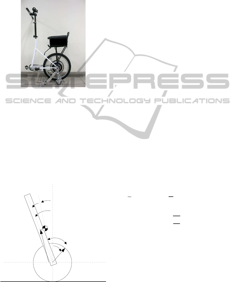
In this paper, a novel, motor-driven, personal mo-

bility vehicle, named Legway, is proposed. As shown

in Fig. 1, Legway is structurally similar to a pedaled

unicycle but with two small auxiliary wheels on the

sides of the main driving wheel. The main driving

wheel is itself a brushless DC (BLDC) hub motor.

The rider can drive Legway forward either electri-

cally by electrical throttle or manually by pedaling it

as the conventional bicycle. The electric driving and

the manual driving can be exercised simultaneously

for the sake of saving the man power or the electric

power. The steering of Legway is achieved by brak-

ing the left auxiliary wheel (for turning left) or the

right auxiliary wheel (for turning right).

Due to the unique driving method, the control de-

sign for Legway requires a special attention. When

the rider pedals, not only the pedalling torque from

the rider but also the controlled torque from the motor

are applied simultaneously on the vehicle. To ensure

efﬁcient operation, it is crucial that these two torques

achieve coordination that they do not interfere with or

ﬁght against each other. In order to reduce the inter-

ference and provide a better human-machine interac-

tion, a novel balancing controller with adaptation ca-

pability is proposed. This balancing controller, when

working together with a specially designed BLDC

motor driver, can adapt to the uncertain center of grav-

ity of the vehicle plus the rider during the pedalling,

and automatically slews the vehicle frame to a balanc-

ing posture depending on the amount of assistive mo-

tor torque demanded. In such a posture, the amount

of motor torque that ﬁghts against the pedaling torque

is reduced to minimum.

This paper investigates the modeling and control

issues of Legwayand is organized as follows: Section

2 shows the system model which includes the mech-

anism dynamics and the motor dynamics. A motor

driveris particularly introduced to properly switch the

modes of operation of the BLDC motor so that a con-

sistent representation of the motor dynamics can be

achieved. In Section 3, a new balancing controller

is proposed and a stability theorem is given to design

120

Huang C. and Yeh T..

Control of a Pedaled, Self-balanced Unicycle with Adaptation Capability.

DOI: 10.5220/0005057801200126

In Proceedings of the 11th International Conference on Informatics in Control, Automation and Robotics (ICINCO-2014), pages 120-126

ISBN: 978-989-758-040-6

 2014 SCITEPRESS (Science and Technology Publications, Lda.)

the control matrices in the controller. Simulations are

performed in Section 4 to verify the usefulness of the

control system. Finally, conclusions are given in Sec-

tion 5.

Figure 1: Photo of Legway.

2 SYSTEM DESCRIPTION

2.1 Model of Legway

Legway’s movement is mainly dictated by its motion

in pitch direction. The pitch dynamics can be charac-

terized by a WIP model in Fig.2. In the model shown,

and I

respectively denote the mass and inertia of

the wheel, m

and I

respectively denote the mass and

inertia of the pendulum body (which includes the ve-

hicle frame and the rider all together), r is the wheel

wheel

, I

)

body

, I

)

Figure 2: Schematics of the wheeled inverted pendulum

(WIP) model.

radius, l is the distance from the wheel axle to the

center of gravity (COG) of the pendulum body, θ

the absolute rotation angle of the wheel, θ

is the ab-

solute inclination angle of the COG of the pendulum

body, θ

is absolute inclination angle of a ﬁxed spot

on the vehicle frame where the tilt sensor is attached

and φ ≡ θ

− θ

is the angular difference between θ

and θ

, τ

is the relative mechanical torque between

the pendulum body and the wheel that τ

consists of

the motor torque τ

, and the rider’s pedaling torque

. It should be noticed that φ could be a time-varying

quantity due to the rider’s posture change during the

riding.

Using the Lagrange formulation, one can derive

the dynamic equation as:

H(q)

q+ C(

q,q)

q+ g(q) = τ (1)

where

q =





τ =



(τ

+ τ

) (τ

+ τ

)



H(q) =



+ m

−m

lrc

−m

lrc

+ (m

+ m



q,q) =



0 0

lrs



, and

g(q) =



−m

gls



. Notice that in the

expressions for H(q) , C(

q,q) , and g(q) , s

and c

are the abbreviations for sinθ

and cosθ

respectively.

The dynamic equation indicates that the min-

imum number of states required to describe the

system is three and the state vector is chosen as





. Equation (1) can be linearized

around the equilibrium state



0 0 0



with τ

= 0, and the linearized state equation is given by:





δθ









0 1 0

αλ

0 0

0 0 0









δθ











α+γ

β+γ







(δτ

+δτ

)

(2)

where, α = I

+ (m

+ m

, β = I

+ m

, γ =

lr, λ = m

gl, η = αβ − γ

. In (2), δ represents the

perturbation around the equilibrium state. For sim-

plicity, the symbol δ will be ignored in the subsequent

discussion.

2.2 Motor Dynamics and Motor Driver

As revealed by the eigenvalues of the system matrix

in (2), the pitch dynamics of Legway is open-loop un-

stable. Moreover, the state equation therein can be

ControlofaPedaled,Self-balancedUnicyclewithAdaptationCapability

121

used to verify that the system is controllable under

the motor torque τ

. Therefore, τ

can be used to not

only stabilize/balance the vehicle but also act as an al-

ternative source of propulsion to the rider’s pedaling

torque.

The motor torque, which is generated by a BLDC

hub motor, is regulated by controlling the motor cur-

rent via a motor driver. Since both positive torque or

negative torque for a wide range of rotational speed

is needed for balancing, accelerating or decelerating

the vehicle, the motor driver devised for this research

can automatically switch between the motoring mode

and the regeneration mode for the sake of energy ef-

ﬁciency. The motor driver also provides a simple,

consistent motor dynamics regardless of the mode

switching.

The switching module in the motor driver as pro-

posed in (Wu and Yeh, 2013) is adopted here. This

module determines which mode the motor should be

switched to for proper operation. Furthermore, to fa-

cilitate the subsequent control design, it also performs

an input transformation so that a single 1st order dif-

ferential equation in the form of

+ Ri = u (3)

can describe the current dynamics for all the four

modes. According to (3), the input to the differen-

tial equation, consequently the switching module is u.

How the mode of operation is selected and how the

duty ratios for PWM switching are computed from

the input u, the measured coil current (i), and the ro-

tational speed (ω) are given in (Wu and Yeh, 2013).

3 BALANCING CONTROL

In Legway, the COG of the vehicle body is dictated by

the rider’s posture and is uncertain to the control sys-

tem. The successful operation of Legway requires the

control system to adaptively estimate the uncertain

COG, slew it to a balanced position and then main-

tain the motor torque at a commanded value. When

the torque command is zero, the COG is slewed to

the top of the wheel axle so that the rider feels mini-

mum interference from the motor as he/she pedals the

vehicle. The rider also does not have to worry about

the uncontrollable acceleration of the vehicle even if

he/she has yet learned to properly place his/her COG

when he ﬁrst rides the vehicle. In the case that the

commanded torque is nonzero, the motor produces an

assistive torque for climbing hills, or stopping the ve-

hicle via regenerative braking.

3.1 Controller Design

The state equation and the output equation for the

controller design are in the form of

˙x = Ax+ Bu+ B

(4)

y = x+ Cϕ (5)

where x,u,y are respectively the state, the input, and

the output vectors, ϕ represents the output distur-

bance, and A, B, C are system matrices. The state

equation, which uses x =





as the state

vector and u =u, is obtained by concatenating the dy-

namics of θ

and

in (2) with the current dynamics

in (3) via τ

= k

i, so A=





0 1 0

αλ

α+γ

0 0 −





,B =













α+γ





. Notice that because it is up

to the rider to apply the pedaling torque or the current

command to control the wheel speed, in the controller

design

is not considered as a state variable. As for

the the output y, it consists of the measured pitch an-

gle (θ

) and the pitch rate (

) from the inclinometer

and the rate gyro installed on the vehicle frame

, and

the motor current (i) from the hall sensors in the mo-

tor. It is assume that the the rider’s posture remains

relatively ﬁxed to the vehicle frame, so φ = θ

− θ

constant and

φ =

−

= 0. This gives ϕ =φ,and

C =



1 0 0



The control objective is to use the feedback from

y to devise a control law for u to make x asymptot-

ically converge to a reference state x

. The major

challenge here is that the output is contaminated by

unknown output disturbance ϕ, so an adaptive scheme

is required for the control system to on-line estimate

and then cancel ϕ. In the following investigation,

we will temporarily ignore τ

, and pose the control

problem in a more general setting for x ∈ R

, u ∈ R

and ϕ ∈ R

which correspond to A ∈ R

n×n

, B ∈ R

n×p

and C ∈ R

n×q

. The controller design for the general

problem is given in the following theorem.

Theorem 1: Given the system in (4)(5) with τ

0, and ϕ being an unknown, constant output distur-

bance, assume that A is invertible, (A,B) control-

lable, and C has full rank. The control system con-

taining

u = −K(ˆx− x

) + u

(6)

is measured directly from the rate gyro. However,

to increase the sensing bandwidth, the measurement for θ

is obtained by merging the outputs of the rate gyro and

the inclinometer using a complementary ﬁlter(T.-J. Yeh and

Wang, 2005).

ICINCO2014-11thInternationalConferenceonInformaticsinControl,AutomationandRobotics

122

as the control law, and

ϕ = −K

(ˆx− x

) (7)

as the estimation law can make x asymptically con-

verge to a reference state x

. In (6) and (7),

ϕ is the

estimation for ϕ, ˆx is the estimated state vector and is

computed by y − C

ϕ, x

is a constant reference com-

mand and u

is the corresponding feedforward con-

trol and both of which should satisfy the structural

constraint

+Bu

= 0, (8)

K is the state feedback matrix which makes A

, where

= A− BK is the nominal closed-loop system ma-

trix, a stable matrix, and ﬁnally K

is the estimator

gain matrix which is computed via the following pro-

cedure:

1. Choose Q

= Q

> 0, Q

= Q

> 0. Com-

pute the solution R = R

> 0 to the Lyapunov matrix

equation

+ A

R = −Q

< 0 (9)

and then the matrix

S= (Q

−1

)

+RBK. (10)

Make sure S is invertible by choosing a ”sufﬁciently

small” Q

or ”sufﬁciently large” Q

2. Deﬁne

D = I

n×n

−SC(C

SC)

−1

(11)

W = C(C

SC)

−1

(12)

and choose Q

= Q

> 0. Compute P, the solution to

the following Riccati equation:

−1

)

P+ P(D

−1

+P(W+ W

)P = −Q

< 0.

(13)

3. K

is computed by

= (C

SC)

−1

P ∈ R

q×n

(14)

Proof. Using a Lyapunov function given by

V = (ˆx− x

)

P(ˆx− x

) +

ϕ+

˜x

(15)

one can prove that ˜x → 0, and

ϕ → 0.

4 SIMULATIONS

The proposed balancing controller is designed based

on the linearized model of Legway. It is then applied

to the nonlinear model consisting of the mechanism

dynamics in (1) and motor dynamics in (3), and the

control performance is examined using simulations.

Table 1: Parameters of Legway model used in the simula-

tion.

Mechanical part Motor part

6 kg R 0.37 Ω

0.0927 kg-m

L 0.503 mH

r 0.25 m k

1.11186 N-m/A

88 kg l 0.85 m

17.6983 kg-m

The system parameters for simulations are listed in

Table 1.

The control gain K, which is de-

signed using LQR method, is given by

K =



419.538 67.835 0.0229



. By choosing

= 1× 10

−8

, Q

= I

and Q

= 7×10

−5

, R and

P are solved, and the estimator gain matrix is given

by K



15.9391 2.7042 9.5750× 10

−4



The closed-loop poles for this design are − 3.577,

−8.648 + 9.089i, −8.648− 9.089i, and −744.34 .

In the simulation, the performance of the pro-

posed controller is compared to two other controllers

respectively referred to as Controller A and Con-

troller B. Controller A uses the measured, biased

states for feedback so that u = −Ky. Controller

B is the one mentioned in Remark 5 and is given

by u = −K

′

y−k

˜ıdt in which the controller gains

′



472.827 67.835 0.0149



and k

= 5.86

are chosen to make the closed-loop poles identical to

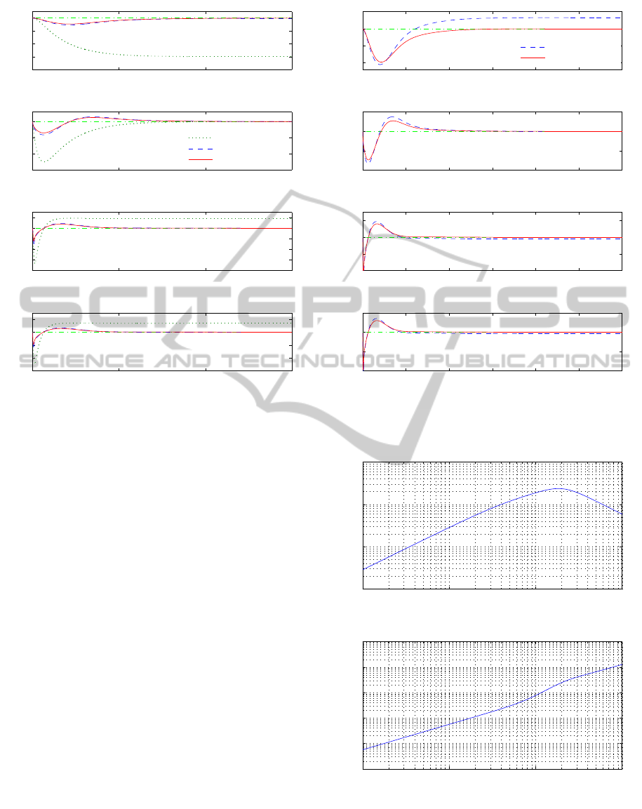
those of the proposed controller. The ﬁrst simulation

assumes that initially x=





= 0. It is

desired to maintain x = 0 (by letting x

= 0 ) under

a constant output disturbance φ = 5

◦

. Fig.3 shows

the responses associated with the states (θ

, i) and

the control (u) for the three controllers. All three

controllers can stabilize the system, but Controller

A, because the lack of estimation capability, exhibits

steady errors in θ

(≈ − 5.994

◦

) and i(≈ 18.53A). On

the other hand, the integral action allows both Con-

troller B and the proposed controller to reject the out-

put disturbance so the state errors all settle to zero

within 1sec. It should be noted that for Controller A,

the steady state error in i results in a constant motor

torque acting on the wheel which in turn causes an

undesired acceleration to the vehicle.

To make furtherperformancecomparison between

Controller B and the proposed controller, a constant

bias of 1A is injected to the current measurement. As

The magnitude of Q

(•)

is quantiﬁed in terms of the ma-

trix norm.

Due to the fact that the magnitude of i in Amps is

much larger than the magnitudes of θ

and

respectively

in radians and radians per second, the third component of

is much smaller than its ﬁrst two components.

ControlofaPedaled,Self-balancedUnicyclewithAdaptationCapability

123

0 0.5 1 1.5

−8

−6

−4

−2

Time (s)

(a) Angle of COG ( θ

)

(deg)

0 0.5 1 1.5

−30

−20

−10

Time (s)

(b) Rate of COG (d θ

/dt)

dθ

/dt (deg/s)

0 0.5 1 1.5

−80

−60

−40

−20

Time (s)

i (A)

0 0.5 1 1.5

−30

−20

−10

Time (s)

(d) Control input (u)

u (V)

Controller A

Controller B

Proposed Controller

Figure 3: Responses of θ

, i, and vehicle speed for the

placement and removal of an 8kg deadweight.

shown in Fig.4, Controller B. which integrates i solely

for integral control, is sensitive to the measurement

bias in i and exhibits steady errors in θ

(≈ 0.324

◦

)

and i(≈ −1.0A). Although the proposed controller

does not explicitly consider the current bias in the de-

sign process (i.e., C=



1 0 0



), the integration

overall the states in the estimator does provide robust-

ness to not only the measurement bias in θ

but also

the bias in i, and all the states reach zero at steady

state.

During manual pedaling, τ

exists and φ could

be a time-varying quantity. They induce a motor

torque even if i

= 0. It is crucial that the control

system keeps the induced motor torque small to avoid

its interference to the pedalling action. To investigate

the inﬂuence of τ

and φ on the motor torque for the

proposed controller, the closed-loop magnitude re-

sponses of the motor torque (k

i) with respect to τ

and φ for the linear model are plotted in Fig.5. It can

be seen that both plots exhibit a high-pass ﬁltering na-

ture, and in particular, the motor torque response due

to τ

has a 0dB crossover frequency around 0.4Hz.

Therefore, as long as τ

and φ are varied slowly, the

induced motor torque is kept small, so the rider can

pedal the vehicle with little interference from the mo-

tor.

0 0.5 1 1.5 2 2.5 3

−1

−0.5

0.5

Time (s)

(a) Angle of COG ( θ

)

(deg)

0 0.5 1 1.5 2 2.5 3

−10

−5

Time (s)

(b) Rate of COG (d θ

/dt)

dθ

/dt (deg/s)

0 0.5 1 1.5 2 2.5 3

−20

−10

Time (s)

i (A)

0 0.5 1 1.5 2 2.5 3

−10

−5

Time (s)

(d) Control input (u)

u (V)

Controller B

Proposed Controller

Figure 4: Responses of θ

, i, and vehicle speed for the

placement and removal of an 8kg deadweight.

−2

−1

−2

−1

f (Hz)

(a) Magnitude response of k

i with respect to τ

| k

i /τ

−2

−1

f (Hz)

(b) Magnitude response of k

i with respect to φ

| k

i /φ | (N/rad)

Figure 5: Responses of θ

, i, and vehicle speed for the

placement and removal of an 8kg deadweight.

ICINCO2014-11thInternationalConferenceonInformaticsinControl,AutomationandRobotics

124

5 CONCLUSIONS

In this paper, a pedaled, self-balanced, personal mo-

bility vehicle, Legway, is developed. The vehicle is

intended to be used in densely populated urban en-

vironments that one can integrate it with the pub-

lic transportation system to increase the commuting

range. In order to reduce the interference and pro-

vide a better human-machine interaction, a novel bal-

ancing controller with adaptation capability is pro-

posed. This balancing controller, when working to-

gether with a specially designed low-level BLDC

driver, can adapt to the uncertain center of gravity of

the vehicle frame plus the rider, and the amount of

motor torque that ﬁghts against the pedaling torque

can be reduced to minimum. The performance of the

control system is validated by simulation.

ACKNOWLEDGEMENTS

The authors gratefully acknowledgethe supports from

National Science Council and National Tsing Hua

University in Taiwan.

REFERENCES

Honda (2009). U3-x. http://asimo.honda.com/innovations/

U3-X-Personal-Mobility/.

Kamen, D. (2001). Segway. http://www.segway.com/.

Polutnik, A. (2006). Enicycle. http://enicycle.com/.

T.-J. Yeh, C.-Y., S. and Wang, W.-J. (2005). Modeling and

control of a hydraulically-actuated inertial platform.

Control Engineering, 219(6):405–417.

Toyota (2008). Winglet. http://www.toyota.com.hk/

innovation/personal

mobility/winglet.aspx.

Wu, F.-K. and Yeh, T.-J. (2013). Drive-by-wire and electri-

cal steering control of an electric vehicle actuated by

two in-wheel motors. Mechatronics, 23(1):46–60.

APPENDIX

This is the proof for the negative deﬁniteness of

Taking time derivative on the Lyapunov function

candidate V in (15) yields

V = 2

ˆx

P(ˆx− x

) + 2

ϕ+2

˜x

··

˜x

= 2˙x

P(ˆx− x

) + 2[−P(ˆx− x

) + Q

ϕ]

+2˙x

RBKC

ϕ+ 2

˜x

in which the second equality is due to

ˆx = ˙y− C

ϕ =

˙x− C

ϕ and differentiating the closed-loop dynamic

equation for the expression of

··

˜x. Notice that

˙x− A

(ˆx− x

) =

˜x− A

(˜x−C

ϕ)

= A

˜x+ BKC

ϕ−A

(˜x−C

ϕ)

= (BK+A

ϕ =AC

ϕ,

(16)

so C

ϕ =A

−1

[˙x− A

(ˆx− x

)]. Replacing C

ϕ by

such an expression,

V becomes

V = 2˙x

P(ˆx− x

)



−1

˙x− (Q

−1

+P)(ˆx− x

)



+2˙x

RBKC

ϕ+ 2

˜x

= 2˙x

P(ˆx− x

)

+2˙x



−1



+ RBK

−2(ˆx− x

)

−1

+P)

ϕ+2

˜x

= 2˙x



P(ˆx− x

) + SC



−2(ˆx− x

)

−1

+P)

ϕ+2

˜x

where the third equality is due to the deﬁnition of

S in (10).

By the estimation law in (7), the deﬁnition of K

in (14), and ϕ being constant, the dynamics associated

with

ϕ is given by

ϕ=

ϕ−

ϕ =

ϕ = −(C

SC)

−1

P(ˆx− x

(17)

Replacing

ϕ in

V by the expression in (17), and then

using the deﬁnitions of D and W respectively in (11)

and (12),

V can be written as

V = 2˙x

DP(ˆx− x

)

+2(ˆx− x

)

−1

+P)

WP(ˆx− x

)

˜x

= 2(ˆx− x

)

D+ (Q

−1

+P)

P(ˆx− x

)

DP(ˆx− x

) + 2

˜x

where the second equality is obtained by substi-

tuting the relation ˙x = A

(ˆx− x

) + AC

ϕ as implied

in (16).

Since

D = C

−C

SC(C

SC)

−1

= C

−C

= 0

V can be further reduced to

V = 2(ˆx− x

)

−1

)

+PWP](ˆx− x

) + 2

˜x

ControlofaPedaled,Self-balancedUnicyclewithAdaptationCapability

125

The property of a quadratic form allows one to expand

V as

V = (ˆx− x

)

−1

)

+P(D

−1

+P(W+ W

(ˆx− x

)

˜x

(RA

˜x,

(18)

so according to the deﬁnitions of P and R respectively

in (13)and (9),

V eventually becomes

V = −(ˆx− x

)

(ˆx− x

) −

˜x

= −(˜x−C

ϕ)

(˜x−C

ϕ) −

˜x

(19)

Since Q

> 0,

V ≤ 0. Furthermore,

V =

0 if and only if ˜x = C

ϕ, and

˜x= 0. From

the closed-loop system equations,

˜x= 0 gives

˜x+ BKC

ϕ = 0, and with ˜x = C

ϕ, one can infer

that (A

+ BK)C

ϕ = AC

ϕ = 0. The invertibility of

A and full rank condition of C lead to

ϕ = 0, which

also means ˜x = 0 . Consequently, the necessary and

sufﬁcient condition for

V = 0 is equivalent to ˜x =0,

and

ϕ = 0. This concludes that

V is negative deﬁnite.

ICINCO2014-11thInternationalConferenceonInformaticsinControl,AutomationandRobotics

126