
Robot Dynamic Model Identification Through Excitation Trajectories
Minimizing the Correlation Influence among Essential Parameters
Enrico Villagrossi
1,2
, Giovanni Legnani
2
, Nicola Pedrocchi
1
, Federico Vicentini
1
,
Lorenzo Molinari Tosatti
1
, Fabio Abb
`
a
3
and Aldo Bottero
3
1
Institute of Industrial Technologies and Automation, National Research Council, via Bassini 15, 20133 Milan, Italy
2
University of Brescia, Dep. of Mechanical and Industrial Engineering, via Branze 39, 25123 Brescia, Italy
3
COMAU Robotics, via Rivalta 30, Grugliasco (TO), Italy
Keywords:
Industrial Robot Dynamics Identification, Optimal Excitation Trajectories, Dynamics Decoupling.
Abstract:
Robot dynamics is commonly modeled as a linear function of the robot kinematic state from a set of dynamic
parameters into motor torques. Base parameters (i.e. the set of theoretically demonstrated linearly-independent
parameters) can be reduced to a subset of “essential” parameters by eliminating those that are negligible with
respect to their contribution in motor torques. However, generic trajectories, if not properly defined, couple
the contribution of such essential parameters into the motor torques, actually reducing the estimation accuracy
of the dynamics parameters. The work presented here introduces an index for evaluating correlation influence
among essential parameters along an executed trajectory. Such index is then exploited for an optimal search
of excitatory patterns consistent with the kinematical coupling constraints. The method is experimentally
compared with the results achievable by one of the most popular IRs dynamic calibration method.
1 INTRODUCTION
Model-based strategies have been introduced in in-
dustrial robots (IRs) control since three decades.
Nonetheless, in spite of the vast literature, methods
for the identification of the dynamic parameters still
remain a matter of substantial investigation.
In fact, an a priori knowledge of the robot dy-
namic parameters is often unavailable (e.g. CAD data
obtained from the design data of manipulators) and
weight tolerances of robot links are remarkable due
to the inaccuracy of the casting process (e.g. around
5-10%, mean value provided by different IR manu-
facturer). Additionally, the real friction model identi-
fication is an experimental procedure per se, with pa-
rameters varying along production batches and time.
In pioneering works (Atkeson et al., 1986; Gau-
tier and Khalil, 1988), the analysis of energy models
led to the identification of a base sub-set of parame-
ters (BP) that are observable through the measure of
motor torques and positions. However, (Pham, 1991)
experimentally demonstrated that only a smaller sub-
set of essentials parameters (EP) are really significant,
i.e. their contribution is not influenced by the preci-
sion and the noise of measuring systems. The set of
EP is valid over and can be numerically computed in
the entire workspace (Antonelli et al., 1999).
Figure 1: Identification Trajectories.
Different identification procedures for EP have
been proposed in literature (Wu et al., 2010). In gen-
eral, the common purpose is to identify the set of dy-
namic parameters that minimizes torque prediction er-
rors (see Section 2 for analytical details). The identi-
fication requires an “optimal” trajectory able to excite
to the best of some metrics the torque produced by
the parameters to be identified (Swevers et al., 1997;
Indri et al., 2002; Park, 2006), see Figure 1. The defi-
nition of “most exciting” trajectory is not unique, and
three main issues have to be faced: (i) the identifica-
475
Villagrossi E., Legnani G., Pedrocchi N., Vicentini F., Molinari Tosatti L., Abbà F. and Bottero A..
Robot Dynamic Model Identification Through Excitation Trajectories Minimizing the Correlation Influence among Essential Parameters.
DOI: 10.5220/0005060704750482
In Proceedings of the 11th International Conference on Informatics in Control, Automation and Robotics (ICINCO-2014), pages 475-482
ISBN: 978-989-758-040-6
Copyright
c
2014 SCITEPRESS (Science and Technology Publications, Lda.)

tion of metrics for evaluating the excitation capabil-
ity; (ii) the consistent comparison of trajectories with
different time-spans; (iii) the selection of the class of
trajectory to be used for robot dynamic excitation.
About the metrics, two indexes (and their com-
binations) are mainly used for quantifying the exci-
tatory power (Presse and Gautier, 1993; Pukelsheim,
2006; Wu et al., 2010): the determinant of the dy-
namic regressor (i.e. estimation with minimal uncer-
tainty bounds); the conditioning number of the dy-
namic regressor (for minimizing the bias of estimates
due to un-modeled dynamics errors). Such kind of
metrics derive from standard mathematic techniques
used in the analysis of observability of linear systems.
However, these methodologies do not allow to over-
come the limitations in observability of EP (Gautier
and Venture, 2013). In fact, both metrics could be
ideally reliable in case of constant uncorrelated exci-
tation of parameters along the full trajectory, which is
never the case: for a generic instant time of a generic
trajectory the complete set of the EP should be not
observable, and the coupling of the parameters should
vary during the trajectory execution. The second key-
aspect in trajectory selection, poorly investigated in
literature, is that standard metrics (e.g. the determi-
nant of the regressor) depend on the number of sam-
ples of the trajectory. A common solution consists
in extracting an equal number of points from different
trajectories. However, the coupling in robot dynamics
does not maintain a constant rate, so differently down-
sampled trajectories may fail in reproducing the cou-
pling effects. The selection of trajectory classes has
instead been deeply investigated in literature, because
it is interpreted as the main tool for improving the
estimation procedure. Many examples of trajectories
have been considered for the proper excitation of the
dynamics (e.g. 5
th
order polynomials in (Caccavale
and Chiacchio, 1994), splines in (Rackl et al., 2012),
a combination of cosine and ramp in (Otani and Kak-
izaki, 1993), finite sums of harmonic sine and cosine
in (Swevers et al., 1997), etc.). However, (Villagrossi
et al., 2013) displays the limited extrapolation power
of classes of excitatory trajectories and how the esti-
mation of EP is affected by such classes: estimated
parameters provide a high prediction power only over
trajectories of the same family of those used during
estimation.
The here presented identification method, at-
tempts to overcome all the three issues reported in
the standard methods. First, an index derived from
the conditioning number index (Presse and Gautier,
1993) is introduced for the evaluation of the coupling
effect in robot dynamics along a trajectory. Second,
a scaling factor over the samples size is introduced
for the determinant of the robot dynamics linearized
regressors, in order to align for comparison different
trajectories, preserving all the sampled dynamics.
Last, the excitatory method is an extension of the
approach in (Villagrossi et al., 2013) to the whole
joint workspace. The method employs at identifica-
tion time a template-class of trajectories applied in
most manufacturing tasks, i.e. general trajectories
described by a set of discrete poses to be interpolated
by the built-in IR motion planner on the basis of
global user-tunable parameters (fly-by accuracy,
velocity profiles, etc.)
1
.
Notation
q =
q
1
,..,q
do f
t
: Joint positions.
q
t
k
,
˙
q
t
k
,
¨
q
t
k
,τ
τ
τ
t
k
: Joint Positions Velocities, accelera-
tions, torques at k-th sample time.
˜
(·),
ˆ
(·), (·)
∗
: Measured, estimated value and opti-
mum estimation respectively.
(·)
+
: is the Moore-Penrose Pseudo-inverse.
2 PROBLEM FORMALIZATION
The robot dynamics at time t
k
is commonly re-
duced (Gautier and Khalil, 1988) to:
τ
τ
τ
t
k
= φ
φ
φ
¨
q
t
k
,
˙
q
t
k
,q
t
k
π
π
π, (1)
where π
π
π is the set EP and matrix function φ
φ
φ is a gener-
alized accelerations. π
π
π includes only combination of
parameters that are experimentally observable along
any excitatory trajectory that generates φ
φ
φ. The min-
imal size N
π
of π
π
π depends on the robot kinematic
topology (Presse and Gautier, 1993; Antonelli et al.,
1999). In addition, other N
f
coefficients of the friction
model yield the compound parameters set π
π
π. The se-
lected friction model (Indri et al., 2002) provides the
j-th joint friction torque function of three parameters,
f
j
0
, f
j
1
, f
j
2
as:
τ
j
f
= f
j
0
sign( ˙q
j
) + f
j
1
˙q
j
+ f
j
2
sign( ˙q
j
)
˙q
j
2
.
For a trajectory of S-samples eq. (1) is expanded as:
T
S
≡
τ
τ
τ
t
1
.
.
.
τ
τ
τ
t
S
=
φ
φ
φ(
¨
q
t
1
,
˙
q
t
1
,q
t
1
)
.
.
.
φ
φ
φ(
¨
q
t
S
,
˙
q
t
S
,q
t
S
)
π
π
π = Φ
Φ
Φ
S
π
π
π, (2)
where Φ
Φ
Φ
S
is the trajectory full regressor matrix. Ac-
tually, experimental sampling
e
T and
e
Φ
Φ
Φ includes also
measurements noise, so that eq. (2) is expressed as:
e
T
S
=
e
Φ
Φ
Φ
S
ˆ
π
π
π +ν
ν
ν, ν
ν
ν ∼ N (0,σ
ν
). (3)
1
COMAU ORL library (COMAU Robotics, 2010) has
been used for the motion interpolation.
ICINCO2014-11thInternationalConferenceonInformaticsinControl,AutomationandRobotics
476

Several techniques are known (Benimeli et al., 2006)
for a pseudo-inversion solution of eq. (3). The
weighted least-squares technique as in (Gautier,
1997) has been here implemented. Denoting W
W
W as
a suitable weight matrix (computed from the standard
deviation of measured torques), the system is solved
as:
ˆ
π
π
π =
h
(
e
Φ
Φ
Φ
t
S
W
W
W
e
Φ
Φ
Φ
S
)
−1
e
Φ
Φ
Φ
t
S
W
W
W
i
e
T
S
. (4)
3 DECOUPLED DYNAMICS
IDENTIFICATION
The method here presented implements a GA for the
identification of “best” exciting trajectories. The fit-
ness function provides two terms similarly to what
proposed in (Presse and Gautier, 1993): one pro-
portional to the logarithm of the determinant of
det
Φ
Φ
Φ
t
S
Φ
Φ
Φ
S
, and one proportional to the coupling in-
dex introduced in the next Section.
3.1 Dynamics Coupling Evaluation
Index over Trajectory
A metric for the evaluation of the coupling effects
along all the path can be straightforwardly derived
from the analysis of conditioning number of the co-
variance. From eq. (2), and under the assumption that
the regression matrix Φ
Φ
Φ is built with a trajectory free
of noise, and that the torque measurements provides
zero-mean uncorrelated noise, the variance of the EP
results:
σ
σ
σ
2
π
= Φ
Φ
Φ
+
σ
σ
σ
2
T
Φ
Φ
Φ
+
t
Assuming the same variance value σ
n
for the measure
of each motor torque such that σ
σ
σ
2
T
= σ
2
n
I
I
I, the relation
can be simplified as follow:
σ
σ
σ
2
π
= Φ
Φ
Φ
+
σ
σ
σ
2
T
Φ
Φ
Φ
+
t
= σ
2
n
Φ
Φ
Φ
+
Φ
Φ
Φ
+
t
= σ
2
n
(Φ
Φ
Φ
t
Φ
Φ
Φ)
−1
= σ
2
n
Ψ
Ψ
Ψ,
where the matrix Ψ
Ψ
Ψ has been introduced for sake of
simplicity. Notably, as a difference from eq. (4), no
weight is applied. Optimal design of the experiment
should correspond to get the matrix Ψ
Ψ
Ψ equal to diag-
onal matrix. Finally, denote the coupling-index as:
I
c
=
N
π
∑
i=1
N
π
∑
j>i
|ψ
i, j
|
√
ψ
i,i
ψ
j, j
. (5)
Each element of the sum are normalized within [0,1].
In addition, if the two parameters i and j are un-cor-
related the value of ψ
i, j
is zero.
Notably, I
c
= 0 corresponds to a diagonal system,
and, thus, it exists a properly scaled system such
that the conditioning number is equal to 1, i.e.
cond(Φ
Φ
Φdiag(λ
1
,...,λ
N
π
)) = 1. However, the defini-
tion of the proper scaling factors λ
i
needs a good a
priori knowledge of EP (Presse and Gautier, 1993).
In addition, I
c
is mathematically simpler and less sen-
sitive to numerical issues to be calculated than the
conditioning number for trajectories with many thou-
sands of points.
3.2 Comparison of Trajectories with
Different Samples Number
Consider eq. (2) and hypothesize to resample the tra-
jectory adding some other S points temporarily each
one near one of the previous points. Thus:
T
2S
=
φ
φ
φ(
¨
q
t
1
,
˙
q
t
1
,q
t
1
)
.
.
.
φ
φ
φ(
¨
q
t
S
,
˙
q
t
S
,q
t
S
)
φ
φ
φ(
¨
q
t
1
+dt
,
˙
q
t
1
+dt
,q
t
1
+dt
)
.
.
.
φ
φ
φ
¨
q
t
S
+dt
,
˙
q
t
S
+dt
,q
t
S
+dt
π
π
π = Φ
Φ
Φ
2S
π
π
π,
with φ
φ
φ
¨
q
t
k
,
˙
q
t
k
,q
t
k
' φ
φ
φ
¨
q
t
k
+dt
,
˙
q
t
k
+dt
,q
t
k
+dt
. It is
easy to demonstrate that
Φ
Φ
Φ
t
2S
Φ
Φ
Φ
2S
' 2Φ
Φ
Φ
t
S
Φ
Φ
Φ
S
and, consequently, the determinant results:
det
Φ
Φ
Φ
t
2S
Φ
Φ
Φ
2S
' det
Φ
Φ
Φ
t
S
Φ
Φ
Φ
S
2
N
π
.
In general, if any point generates k points we get
det(Φ
Φ
Φ
k S
) ' k
N
π
det
Φ
Φ
Φ
t
S
Φ
Φ
Φ
S
.
Finally, if N N
π
in general the determinant of
Φ
Φ
Φ
t
N
Φ
Φ
Φ
N
evaluated on N points is
det
Φ
Φ
Φ
t
N
Φ
Φ
Φ
N
= aN
N
π
→ a =
det
Φ
Φ
Φ
t
N
Φ
Φ
Φ
N
N
N
π
and so a can be used to compare trajectories sampled
with different points.
3.3 Optimal Trajectory Identification
The template-class of trajectory for solving eq. (4) is
directly provided by a real IR interpolator
2
, as in (Vil-
lagrossi et al., 2013). The input for the algorithm is
the trajectory interpolated (by motion planner func-
tions, MP) from a set of K target via-points in the joint
space:
MP(q
1
,...,q
K
). (6)
2
Many robot producers offer libraries compliant to RCS
standard (Vollmann, 2002) and fork.
RobotDynamicModelIdentificationThroughExcitationTrajectoriesMinimizingtheCorrelationInfluenceamong
EssentialParameters
477
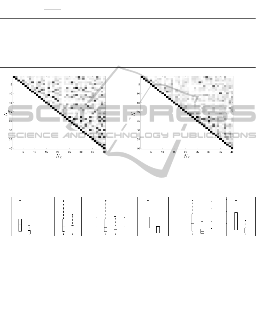
Table 1: GA results (120 generation). N is the samples number. The I
c
for algorithm A has been calculated a posteriori.
N log
10
det(H
t
H)
N
N
π
I
c
Notes
A 2000 90.5 127.9 Eq. (8) in Appendix: W = 3; ω
ω
ω
max
= [0.94,2.38,0.53,0.44,0.89,0.44]
and ω
ω
ω
min
= [0.314,0.314,0.314,0.314,0.314]. GA configuration: num-
ber of individuals=100, mutation=0.01, cross-over rate=0.7. Time dura-
tion of optimization process less than 1 s for each individual.
B 15996 30.9 101.2 Eq. (7): λ
1
= 0.7, and λ
2
= 0.3. Eq. (6): K = 6. GA configuration:
number of individuals=150, mutation=0.01, cross-over rate=0.9. Time
duration of optimization process less than 1s for each individual.
(a) (b)
Figure 2: The figures represent the plot of correlation-matrix defined in equation eq. (5). Black elements are equal to 1 while
color shade to white for elements equal to 0. In figure (a) is shown matrix ψ
i, j
/
√
ψ
i,i
ψ
j, j
obtained from algorithm A while in
figure (b) is shown ψ
i, j
/
√
ψ
i,i
ψ
j, j
matrix obtained from algorithm B. The plot exclude the term related to the friction.
0
50
100
150
Nm
e
A
e
B
(Ax. 1)
0
50
100
150
Nm
e
A
e
B
(Ax. 2)
0
20
40
60
80
Nm
e
A
e
B
(Ax. 3)
0
2
4
6
8
Nm
e
A
e
B
(Ax. 4)
0
5
10
15
20
25
Nm
e
A
e
B
(Ax. 5)
0
5
10
15
Nm
e
A
e
B
(Ax. 6)
Figure 3: Mean error in the torque prediction calculated over 30 randomly wide trajectories covering the whole workspace.
The central mark is the median, the edges of the box are the 25th and 75th percentiles, the whiskers extend to the most extreme
data points the algorithm considers to be not outliers. Trajectories have been generated from the IR Motion Planner.
Individual genomes in the GA are therefore the coor-
dinates of the K via-points and each joint maximum
velocity. The selection of individuals is made on a
two-weighted terms fitness function: the first term is
the D-optimal metric defined in equation eq. (9) and
the second term is the coupling index I
c
in eq. (5):
f = λ
1
log
10
det
˜
Φ
Φ
Φ
t
˜
Φ
Φ
Φ
N
N
π
+ λ
2
I
c
max
I
c
(7)
where I
c
max
is the maximum value of coupling-index,
i.e. I
c
max
= N
π
×(N
π
−1)/2. Fitness terms are nor-
malized so to consistently weight their contributions
through λ
1
and λ
2
in [0,1] such that λ
1
+ λ
2
= 1. A
trial-and-error procedure has been applied for the op-
timal definition of the value of λ
1
and λ
2
.
ICINCO2014-11thInternationalConferenceonInformaticsinControl,AutomationandRobotics
478
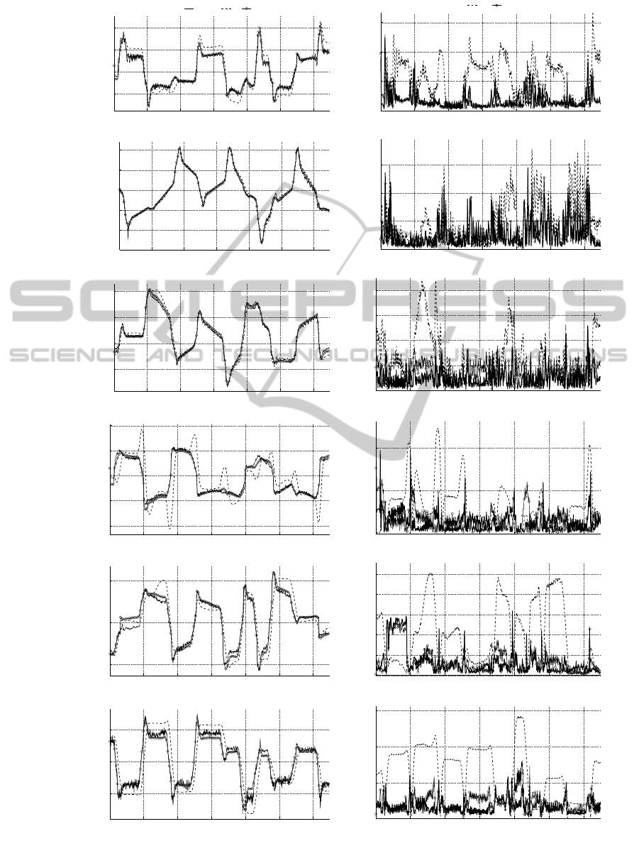
(Ax. 1)
Left:
Values
Right:
Errors
2 4 6 8 10 12
−200
0
200
400
s
Nm
Meas. A B
2 4 6 8 10 12
0
50
100
150
s
Nm
e
A
e
B
(Ax. 2)
Left:
Values
Right:
Errors
2 4 6 8 10 12
−1000
−500
0
500
1000
s
Nm
2 4 6 8 10 12
0
50
100
150
s
Nm
(Ax. 3)
Left:
Values
Right:
Errors
2 4 6 8 10 12
−200
0
200
400
s
Nm
2 4 6 8 10 12
0
20
40
60
80
s
Nm
(Ax. 4)
Left:
Values
Right:
Errors
2 4 6 8 10 12
−40
−20
0
20
40
s
Nm
2 4 6 8 10 12
0
5
10
s
Nm
(Ax. 5)
Left:
Values
Right:
Errors
2 4 6 8 10 12
−50
0
50
s
Nm
2 4 6 8 10 12
0
5
10
15
20
25
s
Nm
(Ax. 6)
Left:
Values
Right:
Errors
2 4 6 8 10 12
−20
0
20
s
Nm
2 4 6 8 10 12
0
5
10
15
s
Nm
Figure 4: Value Measured and Estimated with the two Algorithms A, B for the execution of one sample trajectory of the set
are shown (low pass filter, 30Hz).
RobotDynamicModelIdentificationThroughExcitationTrajectoriesMinimizingtheCorrelationInfluenceamong
EssentialParameters
479

Table 2: Parameters list as in (Villagrossi et al., 2013), an extension of (Antonelli et al., 1999) considering also the 18
parameters of the friction model. π
C
are the data provided from COMAU: from 1 to 40 are the CAD data, while from 41 to
58 are the identified friction values (the parameter from 53 to 58 are zero because COMAU has a linear model of the friction).
COMAU declares a not negligible inaccuracy in the link weight about the 5%-10%.
Par. Id Par. Symb
ˆ
π
∗
A
ˆ
π
∗
B
π
C
Par. Id Par. Symb
ˆ
π
∗
A
ˆ
π
∗
B
π
C
1 mc
2y
1.285 0.499 -0.230 2 I
2xy
-2.241 1.243 0.095
3 I
2yz
-9.113 1.649 -0.053 4 I
3xy
-0.659 1.074 0.100
5 I
3yz
-7.984 0.630 -0.014 6 I
3m
15.465 15.765 10.480
7 mc
4x
0.465 -0.070 -0.001 8 I
4xy
-0.038 -0.521 0.000
9 I
4xz
-1.377 0.295 -0.000 10 I
4m
-6.308 0.878 0.253
11 mc
5x
-0.086 0.020 0.000 12 I
5xy
-2.080 -0.036 -0.000
13 I
5xz
-2.840 -0.029 0.000 14 I
5yz
0.121 0.071 -0.000
15 I
5m
-0.751 3.059 0.298 16 mc
6x
0.186 -0.101 0.001
17 mc
6y
-0.035 0.056 0.000 18 I
6xy
-0.036 -0.023 -0.000
19 I
6xz
-0.901 -0.029 -0.000 20 I
6yz
-0.040 0.023 -0.000
21 I
6zz
0.404 0.029 0.001 22 I
6m
-2.091 1.527 0.120
23 I
1yy
+ I
1m
+ 0.090 m
2
+ I
2yy
+ 0.580 m
3
+ I
3zz
+ 0.614 m
4
+ 0.614 m
5
+ 0.614 m
6
86.800 96.898 79.979
24 mc
2x
+ 0.700 m
3
+ 0.700 m
4
+ 0.700 m
5
+ 0.700 m
6
71.988 71.148 65.056
25 I
2xx
−I
2yy
−0.490 m
3
−0.490 m
4
−0.490 m
5
−0.490 m
6
-50.268 -55.411 -45.728
26 I
2xz
+ 0.700 mc
3y
-3.903 -4.422 2.952
27 I
2zz
+ I
2m
+ 0.490 m
3
+ 0.490 m
4
+ 0.490 m
5
+ 0.490 m
6
102.833 112.234 71.700
28 mc
3x
+ 0.185 m
4
+ 0.185 m
5
+ 0.185 m
6
11.794 10.408 10.725
29 mc
3z
+ mc
4y
+ 0.624 m
5
+ 0.624 m
6
12.770 12.466 12.181
30 I
3xx
−I
3zz
−0.034 m
4
+ I
4zz
+ 0.355 m
5
+ 0.355 m
6
15.805 6.938 2.685
31 I
3xz
−0.185 mc
4y
−0.115 m
5
−0.115 m
6
-1.053 -4.269 -1.606
32 I
3yy
+ 0.034 m
4
+ I
4zz
+ 0.423 m
5
+ 0.423 m
6
4.021 9.244 6.399
33 mc
4z
−mc
5y
-0.036 -0.066 -0.061
34 I
4xx
−I
4zz
+ I
5zz
-2.040 0.558 0.029
35 I
4yy
+ I
5zz
-1.725 -0.131 0.070
36
I
4yz
+ 0.624 mc
5y
-1.013 0.031 0.035
37 mc
5z
+ mc
6z
0.702 0.707 0.190 38 I
5xx
−I
5zz
+ I
6yy
-1.990 -0.066 0.017
39 I
5yy
+ I
6yy
2.474 0.214 0.019 40 I
6xx
−I
6yy
0.644 0.067 0.000
41 f
0,1
38.190 61.121 68.035 42 f
0,2
1.397 0.722 0.719
43 f
0,3
37.803 77.093 108.777 44 f
0,4
2.850 2.479 1.104
45 f
0,5
33.721 37.687 50.446 46 f
0,6
1.497 1.700 0.685
47 f
1,1
4.811 6.262 9.248 48 f
1,2
0.404 0.160 0.057
49 f
1,3
6.232 10.112 8.904 50 f
1,4
0.676 0.277 0.287
51 f
1,5
3.214 0.920 5.148 52 f
1,6
1.117 0.228 0.155
53 f
2,1
-0.005 -0.000 – 54 f
2,2
-0.009 -0.003 –
55 f
2,3
-0.004 -0.003 – 56 f
2,4
-0.010 -0.001 –
57 f
2,5
-0.009 -0.001 – 58 f
2,6
-0.128 -0.001 –
4 EXPERIMENTS AND
DISCUSSION
4.1 Design of Experiment
The experimental setup includes a COMAU NS16
manipulator, with C4GOpen controller option and the
Open Realistic Robot Library. No payload has been
attached. The number of BP for this robot is equal to
43, while EP are 40 (Antonelli et al., 1999). In ad-
dition to inertial parameter, 3 friction parameters per
axis have been considered, yielding a total of N
π
= 58
parameters. The joint positions and the motor cur-
rents have been acquired at 1kHz. The data have been
filtered through approximated spline (MATLAB
(R)
command SPAPS) and tolerance has been set equal to
the measure variance (calculated through ad-hoc ex-
periment). Joint velocities and acceleration have been
calculated as first and second analytical derivative of
the so interpolated joint positions.
As a preliminary investigation of the validity of
the approach, one of the most popular state-of-the-
art methods, (Calafiore et al., 2001), has been im-
plemented and compared experimentally to the one
here proposed. For sake of brevity, “A” and “B” will
be used to indicate the method from (Calafiore et al.,
ICINCO2014-11thInternationalConferenceonInformaticsinControl,AutomationandRobotics
480

2001) and the one here proposed respectively. The
method A is shortly reported in the Appendix for sake
of notation consistency.
4.2 Estimated Parameters
Table 1 reports the characteristics of the two opti-
mal trajectories implemented from the results of the
two algorithms A and B. As expected, A provides a
higher-determinant trajectory, while its coupling in-
dex is poorer. The trajectory from B, in fact, achieves
a much lower correlation influence among EP, see
Figure 2. Both optimal trajectories have been then
executed 30 times each, and the EP have been esti-
mated in each repetition through eq. (4), so that the
EP reported in Table 2 are the mean over the 30 rep-
etitions of the 30 different random trajectories. Fur-
thermore, in Table 2 the fourth column, indicated as
π
C
, lists the CAD data provided from the robot manu-
facturer from 1 to 40 and the friction values identified
from COMAU from 41 to 58 (the parameters from 53
to 58 are zero because COMAU has a linear model
of the friction). COMAU declares a not negligible
variability in the link weight about the 5%-10% due
to the inaccuracy of the casting process. Looking at
parameters from 1 to 22 and from 33 to 58, the Algo-
rithm B identifies values that are averagely closer to
CAD (except parameter 3, 15 and 46). On the other
hand, looking at the parameters from 23 to 32, that are
the complex aggregates parameters, the Algorithm A
identifies values averagely closer to CAD. This dif-
ference should derive from the numerical procedures
used for the EP selection (Antonelli et al., 1999). In-
deed, different thresholds may aggregate BP around
different EP. This should indicate that the method here
presented should be better applied to the identifica-
tion of BP set introducing a priori knowledge of the
system to overcome the issues on the observability.
Future works will be done on this topic.
4.3 Torque Prediction Power
The prediction power of the estimated parameters has
been validated by 30 different random test trajecto-
ries generated through the ORL library. The trajecto-
ries were wide, covering the entire workspace. The
mean error in the torque prediction has been calcu-
lated for each repetition and for each axis. Figure 3
displays the statistics (median/quartile) of the distri-
bution of mean error of each axis over the 30 repe-
titions. Figure 4 displays the results of joint torques
reconstruction for one paradigmatic experiment. Av-
eragely, the algorithm B provide lower prediction er-
ror for all axes.
5 CONCLUSION
The paper has introduced a novel index to estimate the
average coupling of the trajectory in term of correla-
tion among the essential parameters. Two different al-
gorithm have been implemented and compared, test-
ing their performances. Experimental results demon-
strate how a decoupling trajectory produce a better
estimation. Future works will focused on the prop-
agation of the covariance taking into account that the
dynamic regressor Φ
Φ
Φ is not free of noise. Further-
more, a deep analysis of the physical meaning of the
essential parameters will be investigated.
ACKNOWLEDGMENT
R. Bozzi, and J. C. Dalberto, laboratory technicians
of CNR-ITIA, have been involved in setting up the ex-
periments. This work is partially within FLEXICAST
funded by FP7-NMP EC.
REFERENCES
Antonelli, G., Caccavale, F., and Chiacchio, P. (1999).
A systematic procedure for the identification of dy-
namic parameters of robot manipulators. Robotica,
17(04):427–435.
Atkeson, C. G., An, C. H., and Hollerbach, J. M. (1986).
Estimation of inertial parameters of manipulator loads
and links. Int J of Rob Res, 5(3):101–119.
Benimeli, F., Mata, V., and Valero, F. (2006). A compar-
ison between direct and indirect dynamic parameter
identification methods in industrial robots. Robotica,
24(5):579–590.
Caccavale, F. and Chiacchio, P. (1994). Identification of dy-
namic parameters and feedforward control for a con-
ventional industrial manipulator. Control Engineering
Practice, 2(6):1039–1050.
Calafiore, G., Indri, M., and Bona, B. (2001). Robot dy-
namic calibration: Optimal excitation trajectories and
experimental parameter estimation. J. of Robotic Sys-
tems, 18(2):55–68.
COMAU Robotics (2010). Open realistic robot library.
Gautier, M. (1997). Dynamic identification of robots with
power model. In Rob. and Aut., Proc., IEEE Int. Conf.
on, volume 3, pages 1922 –1927.
Gautier, M. and Khalil, W. (1988). On the identification of
the inertial parameters of robots. In Dec and Contr,
Proc. of IEEE Conf. on, volume 3, pages 2264 –2269.
Gautier, M. and Venture, G. (2013). Identification of stan-
dard dynamic parameters of robots with positive def-
inite inertia matrix. In Intell Rob and Sys, 2013
IEEE/RSJ Int Conf on, pages 5815–5820.
Indri, M., Calafiore, G., Legnani, G., Jatta, F., and Visioli,
A. (2002). Optimized dynamic calibration of a scara
RobotDynamicModelIdentificationThroughExcitationTrajectoriesMinimizingtheCorrelationInfluenceamong
EssentialParameters
481

robot. In IFAC ’02. 2002 IFAC Internation Federation
on Automatic Control.
Otani, K. and Kakizaki, T. (1993). Motion planning and
modeling for accurately identifying dynamic parame-
ters of an industrial robotic manipulator. In Proc of
the 24th Int Symp on Ind Rob, pages 743–748.
Park, K. (2006). Fourier-based optimal excitation trajecto-
ries for the dynamic identification of robots. Robotica,
24(5):625–633.
Pham, C. M. (1991). Essential parameters estimation. Dec
and Contr, Proc of IEEE Conf on, 2769(4):2769–
2774.
Presse, C. and Gautier, M. (1993). New criteria of exciting
trajectories for robot identification. In Proc IEEE Int
Conf on Rob and Aut, pages 907–912.
Pukelsheim, F. (2006). Optimal design of experiments. The
Society for Industrial and Applied Mathematics, New
York.
Rackl, W., Lampariello, R., and Hirzinger, G. (2012). Robot
excitation trajectories for dynamic parameter estima-
tion using optimized b-splines. In 2012 IEEE Int.
Conf. on Rob. and Aut., pages 2042–2047.
Swevers, J., Ganseman, C., Tukel, D., de Schutter, J., and
Van Brussel, H. (1997). Optimal robot excitation and
identification. Rob and Aut, IEEE Tran on, 13(5):730
–740.
Villagrossi, E., Pedrocchi, N., Vicentini, F., and Moli-
nari Tosatti, L. (2013). Optimal robot dynamics lo-
cal identification using genetic-based path planning
in workspace subregions. In Adv Intell Mech, 2013
IEEE/ASME Int. Conf. on, pages 932–937.
Vollmann, K. (2002). Realistic robot simulation: multiple
instantiating of robot controller software. In IEEE
ICIT Industrial Technology, volume 2, pages 1194–
1198.
Wu, J., Wang, J., and You, Z. (2010). An overview of dy-
namic parameter identification of robots. Robotics and
Computer-Integrated Manufacturing, 26(5):414–419.
APPENDIX
For sake of clarity, the Appendix reports a brief sum-
mary of the algorithm described in (Calafiore et al.,
2001). Refers to the original paper for all the details.
The template-class of trajectory used for the optimiza-
tion is:
q
j
= q
j
0
+
W
∑
k=1
a
j
k
sin
ω
j
k
t
j = 1,...,do f . (8)
where q
j
0
is the initial offset, a
j
k
and ω
j
k
is respec-
tively the amplitude and the angular frequency of the
sine. W is a small integer representing the maximum
number of harmonics present in the signal. Collect-
ing the free variables a
k
= [a
1
k
,...,a
do f
k
]
t
and ω
ω
ω
k
=
[ω
1
k
,...,ω
do f
k
]
t
, the set of the decision variables of the
optimization problem results {a
1
,ω
ω
ω
1
,...,a
W
,ω
ω
ω
W
}and
proper constraints are to be imposed coherently with
the kinematics of the robot:
|a
j
k
|<
q
j
max
W
, and |ω
j
k
|<
s
¨q
j
max
q
j
max
, j = 1, . . . , do f .
The set of optimum parameters {a
?
1
,ω
ω
ω
?
1
,...,a
?
W
,ω
ω
ω
?
W
}
A
are obtained from the GA. The selection of individuals
is made on the well-known D-optimal considering the
maximization of the determinant of a quadratic form
associated with Φ
Φ
Φ
n
of each n-th individual trajectory
f = log
10
kdet
Φ
Φ
Φ
t
Φ
Φ
Φ
/N
N
π
k. (9)
where N denotes the trajectory samples, and N
π
the
number of the essential parameters. The scaling of
the determinant by the factor N
N
π
has been introduced
in order to allow the comparison between trajectories
with different number of points.
ICINCO2014-11thInternationalConferenceonInformaticsinControl,AutomationandRobotics
482
