
Multi Focus Image Fusion by Differential Evolution Algorithm
Veysel Aslantas and Ahmet Nusret Toprak
Engineering Faculty Computer Engineering Department, Erciyes University, Kayseri, Turkey
Keywords: Multi-focus Image Fusion, Point Spread Function, Differential Evolution Algorithm.
Abstract: In applications of imaging system one of the major problems is the limited depth of field which disallow to
obtain all-in-focus image. However, microscopic and photographic applications desire to have all-in-focus
images. One of the most popular ways to obtain all-in-focus images is the multi focus image fusion. In this
paper a novel spatial domain multi focus image fusion method is presented. The method, firstly, calculates
point spread functions of the source images by using a technique based on differential evolution algorithm.
Then the fused image is constructed by using these point spread functions. Furthermore, the proposed
method and other well-known methods are compared in terms of quantitative and visual evaluation.
1 INTRODUCTION
Obtaining image of a scene can be described as the
projection of 3-Dimensional real world onto 2-
Dimensional image plane. At the end of this process,
it is desirable to have all objects that lying at varying
distances (planes) in the scene, appear to be focused.
However, in practice, cameras that are used in
optical imaging systems are not pinhole devices but
consist of convex lenses. A convex lens can
precisely focus at only one plane of the scene
simultaneously. Therefore, a point object that
located in any other plane is imaged as a disk rather
than a point. However, if the disk, known as the blur
circle, is sufficiently small, it is indistinguishable
from a point, so that a zone of acceptable sharpness
occurs between two planes on either side of the
plane of focus. This zone is named as the depth of
field (DoF). Limited DoF disallows the imaging
systems to obtain all-in-focus images.
One of the most popular ways to extend the
depth of field of an imaging system and to obtain
all-in-focus images is the multi-focus image fusion
that aims gathering information from different focal
planes and fusing them into a single image where
entire objects in the scene appear in focus.
Recently, a huge number of multi-focus image
fusion methods have been proposed. These methods
can be divided into two main groups: transform
based and spatial domain based methods. In former
methods, firstly, a transform is applied on the source
images to get transform coefficients. Then, fusion
process is executed on these coefficients and at last
fused image is acquired by applying inverse
transform. The most commonly used transform
based methods can be given as Laplacian Pyramid
(LP) (Burt and Kolczynski, 1993), Discrete Wavelet
Transform (DWT) (Pajares and de la Cruz, 2004)
and Discrete Cosine Transform (DCT) (Haghighat et
al., 2011). The major disadvantage of these kinds of
methods is that applying a transform before the
fusion stage modifies the original pixel values and
the fusion process is executed on the modified
transform coefficients. This may result in with
unanticipated brightness and color distortions on the
fused images (Li et al., 2013).
On the contrary, the spatial domain based
methods obtain the fused images by directly fusing
the source images due to their spatial features. In the
spatial domain based methods, sharp regions or
pixels are explored to establish the fused image by
transferring these regions or pixels. In the region
based methods the source images are initially
segmented into regions by an appropriate algorithm.
Then, the regions are compared to detect the
sharpest regions. In the pixel based methods, fused
images are generated by detecting the sharpest
pixels. The most known spatial domain methods are
the combination of the sharper blocks by spatial
frequency (Li et al., 2001), combination sharper
blocks by using Differential Evolution algorithm
(Aslantas and Kurban, 2010), region segmentation
and spatial frequency based method (Li and Yang,
2008).
312
Aslantas V. and Nusret Toprak A..
Multi Focus Image Fusion by Differential Evolution Algorithm.
DOI: 10.5220/0005061103120317
In Proceedings of the 11th International Conference on Informatics in Control, Automation and Robotics (ICINCO-2014), pages 312-317
ISBN: 978-989-758-039-0
Copyright
c
2014 SCITEPRESS (Science and Technology Publications, Lda.)

In this paper, a novel spatial domain based multi-
focus image fusion method is proposed. The source
images of the multi-focus image sets consist of both
blurred and focused objects. It is known that the
blurred image of an object can be defined as the
convolution of the focused image of the same object
with a point spread function. From this point of
view, the blurred and the focused pixels of the
source images can be detected by using estimated
point spread functions of the source images. For this
purpose, a novel method that uses Differential
Evolution algorithm to estimate the PSF’s of the
blurred parts of the source images is used in this
paper. The main reason of choosing DE is the
powerful global optimization ability of the
algorithm. Moreover, compared with other
evolutionary optimization methods, DE has some
advantages as being more simple and
straightforward to implement and having fewer
parameters and space complexity (Das and
Suganthan, 2011). The proposed method is
composed of the following steps: firstly, the point
spread functions are calculated over the source
images by using Differential Evolution algorithm.
Then, the focused pixels of the source images are
detected by using estimated point spread functions.
Finally, the detected focused pixels are transferred to
establish the fused image.
This paper is structured as follows. The
proposed image fusion algorithm is described in
section 2. Experimental results are given in section
3. Finally, section 4 concludes the paper.
2 IMAGE FUSION BY
DIFFERENTIAL EVOLUTION
In this section, first, general architecture of the
differential evolution optimization algorithm is
presented. Then the proposed multi-focus image
fusion method is explained.
2.1 Differential Evolution Algorithm
Differential Evolution (DE) is a simple yet powerful
population based, stochastic optimization algorithm
that first introduced by Storn and Price (Storn and
Price, 1997). DE is also a member of evolutionary
algorithms. As an evolutionary algorithm DE uses
mechanisms inspired by biological evolution, such
as reproduction, mutation, recombination and
selection. However, it differs from classical
evolutionary algorithms in producing new
generation of possible solutions by using a greedy
selection scheme. DE often displays better results
than other evolutionary algorithms. The strength of
DE is that it can be easily applied to a wide variety
of real valued problems despite noisy, multi-modal,
multi-dimensional spaces, which usually make the
problems very difficult for optimization.
DE algorithm, firstly, initialize a population of
possible solutions. Then, new populations are
created by using simple mathematical operators to
combine the positions of existing individuals. If the
position of a recently produced individual is an
improvement, then it is included in the population
otherwise the new individual is removed. This
process is repeated for each generation until one of
the stopping criteria (e.g. maximum generation) is
met. The basic steps of DE: initialization of
population, mutation, recombination and selection
are briefly explained in following section.
Initialization of Population: If the function that
wants to be optimized has D real parameters, it can
be represented with a D-dimensional vector. DE
algorithm initializes population of solution with NP
solution vectors. Each parameter vector has the
following form:
,
,,
,
,,
,...,
,,
1,2,...,.
(1)
If there is no prior knowledge about possible
solutions, initial population is produced randomly as
following expression:
,
0,1
(2)
where x
i
H
and x
i
L
are the upper and lower bounds
for each parameter, respectively.
Mutation: Mutation operator is applied to each
parameter of vectors to expand the search space. For
a given target vector x
i,G
, a mutant vector v
i,G+1
generated by combining randomly selected three
vectors of current generation x
r1,G
, x
r2,G
, and x
r3,G
as
follows:
,
,
,
,
(3)
where i, r1, r2 and r3 are distinct random integer
indices and F ∈ [0, 2] is mutation factor.
Recombination: DE utilizes recombination
operator that incorporates successful solutions from
the previous generation in order to increase the
diversity of the population. The new vector u
i,G+1
is
formed by using the target vector x
i,G
and the mutant
vector v
i,G+1
:
,,
,,
i
f
,
or
,,
i
f
,
or
(4)
where j = 1,2,…,D; rand
j,i
∈ [0, 1] is a random
MultiFocusImageFusionbyDifferentialEvolutionAlgorithm
313

number, CR ∈ [0, 1] is called recombination
probability and I
rand
∈ [1,2,…,D] is randomly
selected index that ensures v
i,G+1
≠ x
i,G
.
Selection: The recently produced vector u
i,G+1
is
compared with the target vector x
i,G
in order to
decide which one is included in next generation of
population. The one with the better fitness function
value is selected by following expression.
,
,
i
f
,
,
,
(5)
2.2 Detecting the PSFs of the Source
Images Using DE
Digital imaging systems are suffered from limited
depth of field and this problem lead to obtain images
that consist of both sharp and blurred regions. In
order to obtain all-in-focus image of a scene, multi-
focus images of it obtained from an identical point
of view with different optical parameters can be
used. However, the sharp pixels of these images
need to be properly determined.
The blurred image of an object can be defined as
the convolution of the sharp image of the same
object with the PSF of the camera (Aslantas and
Pham, 2007). If both the sharp and the blurred
images of same object are exists then the PSF can be
computed by a deconvolution process. Objects at
particular distance in the scene are viewed in focus
in one of the source images and out of focus in the
others.
Thus, for all objects, if both of the sharp and
the blurred images are exist, the PSF of blurred
images can be computed by using them.
To explain the theory of the proposed method, a
linear imaging model is used in this paper. Suppose
that i
1
is the near focused and i
2
is the far focused
image of the same scene. Besides, let f represents the
foreground objects and g represents the background
objects of the scene.
(6)
where f
s
and g
s
represent the sharp images and f
b
and
g
b
represent the blurred ones, respectively.
Since the blurred image of an object can be
obtained by convolving the sharp image of the same
object with the PSF of the camera, Eq. 6 can be
written as following:
⊗
⊗
(7)
where h
1
and h
2
are the PSFs. After examining the
several wavelengths and considering the effects of
lens aberrations, the point spread function is best
described by a 2D Gaussian function (Subbarao et
al., 1995).
,
1
2πσ
(8)
where
is the spread parameter (SP).
In order to determine the optimal PSFs of the
source images, the proposed method employs the
DE algorithm. The parameters that are searched in
optimization process are the SPs of the PSFs of the
source images. The steps of detecting the optimal
PSFs can be given as follows:
Step 1: Define the parameters of the DE
algorithm (CR, F, NP) and the termination criteria.
Step 2: Generate the initial population randomly.
Each individual has the parameters as the number of
the source images. In our example, each individual
consist of two parameters σ
1
and σ
2
that denotes the
spread parameters of PSFs of the source images h
1
and h
2
, respectively.
Step 3: Evaluate the population by computing
the fitness function value of each individuals.
Produce estimated PSFs for the source image by
substituting σ
1
and σ
2
in Eq. 8, respectively.
Generate artificially blurred images by
convolving the source images with the each other’s
PSFs. Hence, i
1
is convolved with h
2
and i
2
is
convolved with h
1
to produce c
1
and c
2
images,
respectively as:
⊗
⊗
(9)
Obtain the difference images by subtracting c
2
from i
1
and c
1
from i
2
as:
⊗
⊗
(10)
For the ideal PSFs, the dot product of d
1
and d
2
should be equal to zero. In order to obtain the fitness
value of the each solution, the following expression
is used as the fitness function:
f
σ
,σ
d
.d
(11)
Step 4: In order to generate the next generation
of population, apply the mutation and recombination
operators of DE to current solutions.
Step 5: Repeat the steps 3-4 until a stopping
criteria is met.
2.3 Fusing the Source Images Using the
Optimal PSFs
After estimating optimal PSFs of the source images,
the sharp pixels can be detected by using these. To
ICINCO2014-11thInternationalConferenceonInformaticsinControl,AutomationandRobotics
314

this end, first, the source images are artificially
blurred by convolving with the estimated PSFs (h
1
and h
2
) to compute the artificially blurred images c
2
and c
1
. In c
1
and i
2
, f obtained with the same amount
of blur. Also, the regions corresponding to g in c
2
and i
1
are blurred equally. By making use of this
information, the sharp pixels can be detected.
In order to determine sharp pixels, the difference
images are obtaining by substituting optimal PSFs in
Eq. 10. By optimal PSFs, f and g are cancelled out in
d
1
and d
2
, respectively. At last, each pixel of d
1
and
d
2
are compared to construct the fused image i
F
as:
,
,
,
(11)
3 EXPERIMENTAL RESULTS
This section reports the evaluations of the fusion
results of the proposed method by quantitatively and
visually. In order to evaluate the performance of the
proposed method quantitatively, assessing indexes
Quality of Edges (QE) (Xydeas and Petrovic, 2000)
and Fusion Factor (FF) (Stathaki, 2008) are applied.
The results of the proposed method are compared
with three other well-known methods: Discrete
Wavelet Transform (DWT) (Pajares and de la Cruz,
2004), Discrete Cosine Transform (DCT)
(Haghighat et al., 2011) and block based spatial
domain (BBSD) (Li et al., 2001). For DWT “sym8”
filter and 7 decomposition level are chosen. For
BBSD method block size is selected as 16×16 and
SF is used as sharpness measure. As a result of many
experiments conducted, control parameters of DE is
chosen as CR = 0.6, F = 0.6 and NP = 16 for the
proposed method.
In the experiments, the multi-focus image sets:
“Lab”, “Book” and “Watch” are used. The source
images of these sets are shown in Fig. 1.
Figure 1: The source images used in the experiments.
The first experiment was performed on the “Lab”
source images given in Fig. 1. The fused images and
the difference images that obtained by subtracting
source images from fused images are shown in Fig.
2. It can be seen on the figure, the fused images of
DWT and DCT methods have some artifacts on the
head of the man. If the source images of “Lab”
image set are examined carefully, it can be seen that
head of the man has slightly moved between two
images. This condition leads to artifacts in fused
images of the DWT and the DCT methods that
suffer from shift variance. Although the result of the
BBSD method is satisfactory in this area, it produces
some artifacts in other regions. Especially, it cannot
preserve the form of the clock and introduces some
blocking effects. On the other hand, the fused image
of the proposed method does not contain major
artifacts.
The second experiment was carried out on the
“Book” image set that contains detailed textures.
The fused and the difference images of the “Book”
image set are given in Fig. 3. It can be seen from the
figure, the proposed and the DCT methods have a
good fusion performance on this image set. On the
other hand, the DWT method could not preserve all
the high frequency details and this can be seen more
clearly in the difference images. Moreover, in spite
of producing fewer artifacts than the DWT, the
BBSD method produced some artificial edges
around the borders of books.
The last experiment was performed on the
“Watch” multi-focus image set. Fig. 4 displays the
fused and the difference images of the “Watch”
image set. If the fused images are examined,
intensive distortions on details such as the pin of the
watch can be seen in the DWT and DCT methods.
Similarly, the BBSD method could not preserve
details properly. When the block size cannot fulfill
the little details exactly, the BBSD method cannot
produce perfect fused images for the image sets that
contain too little objects. On contrary, there are no
obvious artifacts in the fused image of the proposed
method.
Table 1 gives the quantitative results of the
methods in terms of the QE and the FF metrics. Bold
values in the table indicate the greater values in the
corresponding column. It can be seen from the table
that the proposed method outperforms the other
methods. Only for the “Book” and the “Watch”
image sets, the DCT method produced better result
than the proposed method in term of FF metric.
However, it can be seen that the proposed method
has very close result to that. Besides, if the “Watch”
fused image of DCT method is examined, blur on
the pin of the watch observed. This situation
demonstrates that in some cases quality indexes have
some significant drawbacks.
MultiFocusImageFusionbyDifferentialEvolutionAlgorithm
315
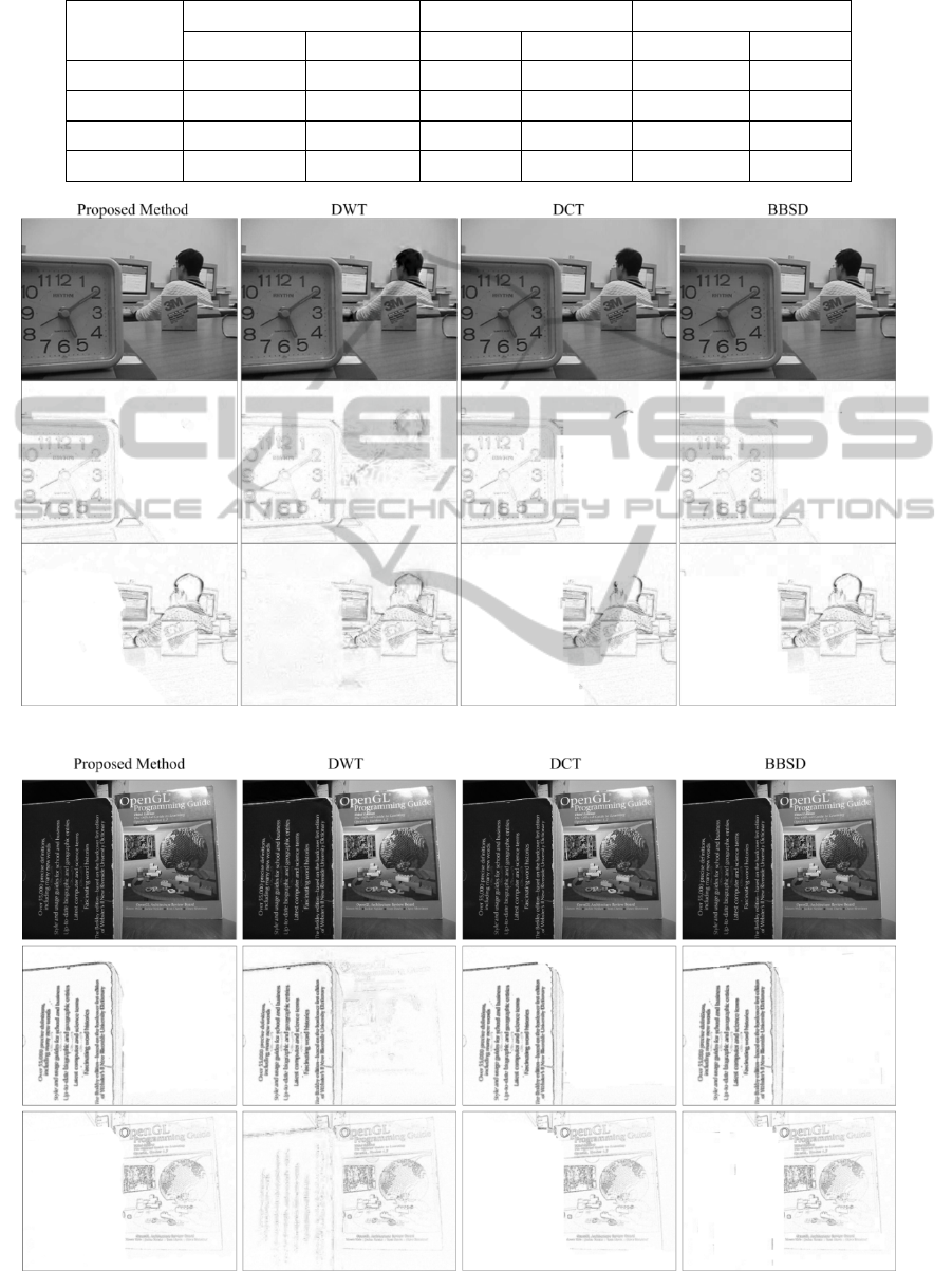
Table 1: The quantitative results of the fusion methods.
L
ab
B
ook
Watc
h
QE
FF
QE
FF
QE
FF
Method
0,7482
9,8998
0,7408
22,5540
0,7221
9,3001
DWT
0,6728
7,1553
0,6881
11,4353
06487
5,6153
DCT
0,7446
9,8627
0,7400
22,9122
0,7167
9,3365
BBSD
0,7478
9,8501
0,7406
22,1375
0,7204
9,2017
Figure 2: The fused and the difference images of the Lab image set.
Figure 3: The fused and the difference images of the Book image set.
ICINCO2014-11thInternationalConferenceonInformaticsinControl,AutomationandRobotics
316
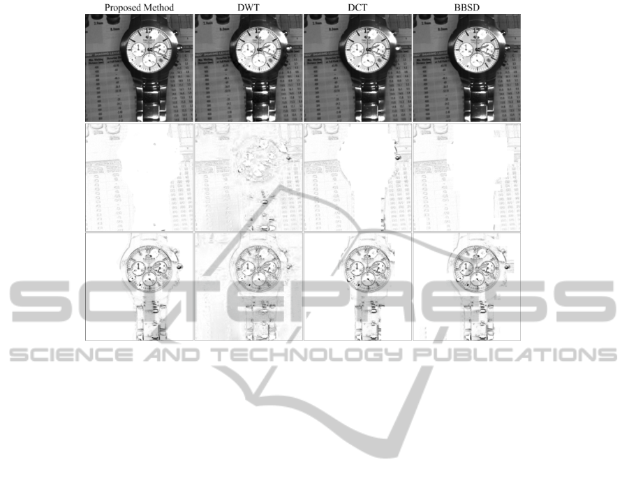
Figure 4: the fused and the difference images of the Watch image set.
4 CONCLUSIONS
In this paper a powerful multi-focus image fusion
technique is proposed for extending image’s
apparent depth of field. The proposed method
estimate PSFs of the source images by using DE
method, and then each image is artificially blurred
by convolving these PSFs. Then, the artificially
blurred images are used to determine the sharpest
pixels of the source images. Finally, the all-in-focus
image of the scene is constructed by gathering the
sharpest pixels of the source images. Also
experimental results are performed on the multi-
focus image sets. These experiments reveal that the
proposed method outperforms over the well-known
DWT, DCT and BBSD methods in terms of both the
quantitative and the visual evaluations.
REFERENCES
Aslantas, V. & Kurban, R. 2010. Fusion Of Multi-Focus
Images Using Differential Evolution Algorithm.
Expert System Applications, 37, 8861-8870.
Aslantas, V. & Pham, D. T. 2007. Depth From Automatic
Defocusing. Optics Express, 15, 1011-1023.
Burt, P. J. & Kolczynski, R. J. 1993. Enhanced Image
Capture Through Fusion. In: Computer Vision, 1993.
Proceedings., Fourth International Conference On, 11-
14 May 1993 1993. 173-182.
Das, S. & Suganthan, P. N. 2011. Differential Evolution:
A Survey Of The State-Of-The-Art. Evolutionary
Computation, Ieee Transactions On, 15, 4-31.
Haghighat, M. B. A., Aghagolzadeh, A. & Seyedarabi, H.
2011. Multi-Focus Image Fusion For Visual Sensor
Networks In Dct Domain. Computers & Electrical
Engineering, 37, 789-797.
Li, S., Kang, X., Hu, J. & Yang, B. 2013. Image Matting
For Fusion Of Multi-Focus Images In Dynamic
Scenes. Information Fusion, 14, 147-162.
Li, S., Kwok, J. T. & Wang, Y. 2001. Combination Of
Images With Diverse Focuses Using The Spatial
Frequency. Information Fusion, 2, 169-176.
Li, S. & Yang, B. 2008. Multifocus Image Fusion Using
Region Segmentation And Spatial Frequency. Image
And Vision Computing, 26, 971-979.
Pajares, G. & De La Cruz, J. M. 2004. A Wavelet-Based
Image Fusion Tutorial. Pattern Recognition, 37, 1855-
1872.
Stathaki, T. 2008. Image Fusion: Algorithms And
Applications, Academic Press.
Storn, R. & Price, K. 1997. Differential Evolution – A
Simple And Efficient Heuristic For Global
Optimization Over Continuous Spaces. Journal Of
Global Optimization, 11, 341-359.
Subbarao, M., Wei, T. C. & Surya, G. 1995. Focused
Image Recovery From Two Defocused Images
Recorded With Different Camera Settings. Image
Processing, Ieee Transactions On, 4, 1613-1628.
Xydeas, C. S. & Petrovic, V. 2000. Objective Image
Fusion Performance Measure. Electronics Letters, 36,
308-309.
MultiFocusImageFusionbyDifferentialEvolutionAlgorithm
317
