
A Time-analysis of the Spatial Power Spectra Indicates the Proximity
and Complexity of the Surrounding Environment
Ana Carolina Silva and Cristina P. Santos
Industrial Electronic Department, University of Minho, Azurem Campus, Guimarães, Portugal
Keywords:
Image Power Spectra, Image Processing, Robotic Control.
Abstract:
In this paper, the statistical properties of both simulated and real image sequences, are examined. The image
sequences used depict different types of movement, including approaching, receding, translation and rotation.
A time analysis was performed to the spatial power spectra obtained for each frame of the image sequences
used. Here it is discussed how this information is correlated to the proximity of the objects in the visual
scene, as well as with the complexity of the environment. Results show how scene and visual categorization
based directly on low-level features, without segmentation or object recognition stages, can benefit object
localization and proximity. The work here proposed is even more interesting considering its simplicity, which
could be easily applied in a robotic platform responsible for exploratory missions.
1 INTRODUCTION
Visual perception is becoming increasingly important
in the robotic field, more specifically on the control of
complex tasks, as autonomous navigation in unstruc-
tured environments, collision avoidance, among other
behaviours. Unfortunatly, vision is an exceptionally
complex task. In light of the difficulties computer vi-
sion research has run into, the computational accom-
plishment of biological visual systems seems all the
more amazing. Biology has solved the task of every-
day vision in a way that is superior to any machine
vision system. Consequently, computer vision scien-
tists have tried to drawn inspiration from biology. A
very promising bio-inspired approach for solving the
difficult problems in vision, is based on the adaptation
to image statistics(Hyvrinen et al., 2009).
Even from a casual inspection of natural images,
which are image scenes captured in a natural areas,
it can be noticed that neighbouring spatial locations
are strongly correlated in intensity. According to lit-
erature (Simoncelli and Olshausen, 2001), the stan-
dard measurement for summarizing these dependen-
cies is the intensity autocorrelation function, which
computes the correlation of the image pixel’s inten-
sity at two locations as a function of their spatial sep-
aration. A closely related measurement is its Fourier
transform, in particular, the image power spectrum.
Expressing the autocorrelation function by its Fourier
transform is convenient for several reasons. It con-
nects the statistics of images with linear systems mod-
els of image processing.
Futhermore, the two-dimensional power spectrum
has usually been reduced to a one-dimensional func-
tion of spatial frequency, by performing a rotational
average on the two-dimensional Fourier plane. Ex-
tensive experimental analysis had lead researches to
find out that the power spectrum of natural images
falls with frequency as 1/ f
α
, being α a value tipically
close to 2. Field (Field, 1987) has shown that natural
images have a so-called self similar power spectrum.
Ruderman and Bialek (Ruderman and Bialek, 1994)
has shown that the self similar power spectrum varies
among different classes of images and, some years af-
ter (Ruderman, 1997), this author has argued that is it
also the particular distribution of sizes and distances
of objects in images that governs the spectral falloff.
In fact, during the last years, there has been a great
deal of interest in the images statistics, both from
a computational and biological vision perspective.
Considering the computational perspective, this inter-
est emerged from: 1) the needing for better redudancy
reduction/image compression and image/video cod-
ing strategies (Buccigrossi and Simoncelli, 1999); 2)
the pursuit for better image restoration algorithms (in-
cluding denoising, inpaiting, among others) (Nielsen
and Lillholm, 2001); 3) the necessity to estimate sur-
faces (depth map) from stereo, texture, motion, shad-
ing (Torralba and Oliva, 2002). From a biological per-
spective, most research has been focused on studying
148
Quintela Alves Vilares da Silva A. and Santos C..
A Time-analysis of the Spatial Power Spectra Indicates the Proximity and Complexity of the Surrounding Environment.
DOI: 10.5220/0005061401480155
In Proceedings of the 11th International Conference on Informatics in Control, Automation and Robotics (ICINCO-2014), pages 148-155
ISBN: 978-989-758-040-6
Copyright
c
2014 SCITEPRESS (Science and Technology Publications, Lda.)

how neural properties (from photoreceptors to visual
cortical neurons) are adapted to the statistics of the
visual environment. Additionally, artificial models of
biological image processing have been developed and
used to verify the influences of ecological niches on
the characteristics of neural receptive fields (Balboa
and Grzywacz, 2003; Field, 1987; Doi et al., 2012).
While the majority of the research in this sci-
entific field has been focus in evaluating the spatial
frequency of images, a full consideration of image
statistics must certainly include time (Hateren, 1993;
Dong and Atick, 1995). Images falling on the retina
have important temporal structures arising from self-
motion of the observer, as well as from the motion of
objects in the world. Despite the complexity of daily
image sequences captured by the biological systems,
natural vision systems appear to work well in complex
3D scenes. Many fast moving animals, either simple
as flies and bees, or more complex biological systems
as birds, seem to have little trouble navigating through
the environments. In fact, vision is concerned with the
perception of objects in a dynamical world, one that
appears to be constantly changing when viewed over
extended periods of time.
Looking at these findings from an engineering
point-of-view, in this paper we illustrate how simple
statistis of simulated and real images vary as a func-
tion of the interaction between the world and the ob-
server. A methodology that highlights those changes
on the statistical properties, according to distance or
scene complexity, is here proposed, which could be
easily implemented in a simple robotic platform. Re-
sults show how simple image statistics can be used
to predict the presence or absence of objects in the
scene, before exploring the image/environment.
For a better understanding of the work here pro-
posed, the paper is organized as follows: in section
2, a brief literature review is performed, in order to
point out important work previously developed in this
scientific field. In section 3, the mathematical formu-
lation of the methodology here proposed is described
in detail, as well as the image sequences developed
and used to test the methodology. In section 4, impor-
tant experimental results are presented. Finally, the
conclusion of the work here described is presented on
section 5.
2 RELATED WORK
The statistical properties of static images have been
studied for many years (Burton and Moorhead, 1987),
seeking to describe the spatial regularities and corre-
lations of such images. However, during those years,
the regularities in time-varying images had been stud-
ied in a very limited way, mainly due to the high cost
associated with the technology to capture and analyse
motion pictures on computers, by then.
Posteriorly, in 1992, van Hateren (Hateren, 1992)
performed the first research aiming to character-
ize, indirectly, the spatio-temporal structure of visual
stimuli. This was determined by the spatial power
spectrum of the natural images, combined with the
distribution of velocities perceived by the visual sys-
tem, when moving in the environment. Through this,
van Hateren was able to infer about the joint spatio-
temporal spectrum obtained for the situations tested
and, subsequently, about the optimal neural filter for
maximizing the information rate in the photorecep-
tive channels of the eye. This analysis enabled van
Hateren to verify the high correlation between the
temporal response properties of biological visual neu-
rons and the optimal neural filter derived from this
study.
In 1995, Dong and Attick (Dong and Atick, 1995)
measured the spatio-temporal correlations for a group
of motion pictures segments, through the computation
of the three-dimensional Fourier transform on these
movie segments and then by averaging together their
power spectra. In Dong and Attick work (Dong and
Atick, 1995), it was shown that the slope of the spatial
power spectrum becomes more flat at higher tempo-
ral frequencies. At the temporal frequency spectrum
domain, the slope becomes more flat at higher spa-
tial frequencies. These results showed that the depen-
dence between spatial and temporal frequencies is, in
general, non-separable. A theorical derivation of this
scaling behaviour was proposed, being demonstrated
that it emerges from objects, with a static power spec-
trum, appearing at a variety of depths and moving
at different velocities relative to the observer. Ad-
ditionally, and similarly to the methodology imple-
mented by van Hateren (Hateren, 1992), Dong and
Attick computed the optimal temporal filter to remove
time correlations. The filter proposed was proved
to closely match the lateral geniculate neurons’ fre-
quency response function.
More recently, Rivait and Langer (Rivait and
Langer, 2007) examined the spatiotemporal power
spectra of image sequences depicting dense motion
parallax, namely the parallax seen by an observer
moving laterally in a cluttered environment. A pa-
rameterized set of computationally generated images
sequences were used and the structure of its spatio-
temporal spectrum was analysed in detail. This work
specifically addressed lateral translation. However,
the analysis here proposed could be generalized to
more complex type of motion, including components
ATime-analysisoftheSpatialPowerSpectraIndicatestheProximityandComplexityoftheSurroundingEnvironment
149

of rotation or forward translation.
In order to summarize distinct work that have been
developed in this research field, in (Pouli et al., 2010)
a deep and detailed review relative to the state of the
art in image statistics was performed. Additionally, its
potential applications on the computer graphics field,
as well as with related areas, was also addressed in
the cited paper (Pouli et al., 2010).
Looking at the potential use of the image power
spectra in a different perspective, Dror et al. (Dror
et al., 2000) and Wu et al. (Wu et al., 2012) ad-
dressed the problem of motion/velocity estimation, by
coupling the output of a well-known bio-inspired el-
ementary motion detector and a real-time computed
image power spectrum. According to the results ob-
tained with this methodology (Wu et al., 2012), the
real-time reliability of velocity estimation was highly
improved.
Taking into account these findings, in this paper a
new methodology, based on a real-time computation
of the image power spectra, is proposed. It is expected
to give an indication about: movement of objects in
the environment; complexity of the surrounding envi-
ronment; safety of the trajectory path.
3 MATERIALS AND METHODS
3.1 Power Spectrum Estimation and
Power Spectrum Fitting Functions
For each frame of the images sequences, either sim-
ulated or real, the methology here proposed starts by
computing the discrite Fourier transform (FT) of each
image, through:
FT
t
( f
x
, f
y
) =
N−1
∑
x=0
N−1
∑
y=0
I
t
(x,y)e
−i
2π
N
( f
x
x+ f
y
y)
(1)
where I
t
(x,y) denotes the intensity of the pixel in
the (x,y) position, at time instant t; f
x
and f
y
denote
the spatial frequencies in x and y directions; N indi-
cates the image size.
The image power spectra (PS) is then computed
through the following way:
PS
t
( f
x
, f
y
) =
|
FT
t
( f
x
, f
y
)
|
2
(2)
Then, by performing a rotational average within
the two-dimensional fourier plane, the power spectra
from equation 2 is reduced to a one-dimensional
function of spatial frequency, f
r
=
√
f
2
x
+ f
2
y
, being
well approximated by the function:
P
t
( f
r
) = A ·
1
f
α
t
r
= A · f
−α
t
r
(3)
where P
t
is linear with slope equal to −α, when
plotted in a loglog scale, and A is an arbitrary con-
stant that depends on scene composition. Accord-
ing to literature, α value depends on many factors,
as image depth , image blurring, sparseness of local
structures, among other characteristics (Torralba and
Oliva, 2002; Ruderman, 1997; Field and Brady, 1997;
Liu et al., 2008).
In order to analyse the cumulative slope variation
across time, and after performing simulations in order
to observe how slope variations were related to char-
acteristics of known and controlled environments, a
further analysis needs to be performed, through:
△α
t
= α
t
− α
t−1
+ △α
t−1
(4)
where,
{
△α
t
= 0, if △α
t
< 0
△α
t
= △α
t
, if △α
t
≥ 0
(5)
The computation of △α for each time instant t,
constitutes an indication about the variations in the
power spectrum slope. Indirectly, it can be an indica-
tor of the object proximity, as well as the environmen-
tal complexity.
3.2 Image Sequences
In the present work, both simulated and captured im-
age sequences have been used. Artificial image se-
quences were created using Matlab. Objects were
simulated according to the specific characteristics re-
quired. Image sequences were captured by a simu-
lated camera with a field of view of 60º in both x and
y axis, a size of 100 × 100 pixels and a sampling fre-
quency of 100 frames per second. This simulated en-
vironment enabled the adjustment of several parame-
ters, such as: image matrix dimensions; camera rate
of acquisition; image noise level; number, size, shape,
texture, distance of objects; contrast; among other
characteristics. Additionally, movement (at different
speeds), as well as trajectories with different com-
plexity levels could be added to the objects present
on the artificial image sequence created.
A looming object, with a specific half lenght l and
moving at a constant speed v, shows a typical rate
of expansion, with a slow initial angular speed that
rapidly increases as the object is getting closer to the
camera. The angular size subtented at the camera by
an approaching object is given by:
θ(t) = 2 · tan
−1
(l/vt) (6)
ICINCO2014-11thInternationalConferenceonInformaticsinControl,AutomationandRobotics
150
in which t denotes the Time-To-Collision (TTC)
of the object in relation to the camera, conventionally
chosen to be negative prior to collision. Velocity is
negative for an object approaching and positive to an
object receding.
In a looming approach, both the angular size (θ(t))
and the angular expansion rate are non-linear func-
tions of time, whose temporal dynamics solely de-
pend on l/|v| ratio. Based on this physical principle,
looming, receding and translating trajectories were
created, for differente l/|v| ratios of the visual stim-
uli.
Thus, this artificial environment enables us to con-
trol all the characteristics of the input data.
Additionally, in order to obtain real video se-
quences, a Pioneer 3-DX robot was placed within a
real lab environment. A PlayStation Eye digital cam-
era was used to capture videos. The resolution of the
video images was 640 × 480 pixels, with an acquisi-
tion frequency of 30 frames per second.
The computer used was a Laptop (Toshiba Portégé
R830-10R) with 4 GHz CPUs and Windows 7 operat-
ing system.
4 RESULTS
In a way to show the feasibility of the method here
proposed, two different experiment types were per-
formed. The first experiment was made on a simu-
lated data set, in which we analyzed the dependency
of: the object size, trajectory, and distance on param-
eter α, from equation 3, and on △α, from equation
4. The second set of experiments were performed in
real image sequences, including the ones captured by
a camera placed on a Pioneer 3DX robot, located in a
real environment, when performing a translational or
a rotational trajectory.
4.1 Artificial Image Sequences:
Looming, Receding and Translating
Trajectories
In order to analyse how the slope of the averaged
power spectra α changes as an object approaches to
the camera (being located, at different time instants,
at different distances to the simulated camera), a sim-
ulated visual stimuli of an approaching square, with
two different sizes (l): 10×10 pixels and 20×20 pix-
els, and a speed (v) of 2 m/s was created. The obtained
results are depicted on figure 1.
Analyzing the obtained results, we can verify that
the slope value of the averaged power spectra (α) as
−0.5 −0.4 −0.3 −0.2 −0.1 0 0.1
−3
−2
−1
0
Slope of the averaged
Power spectra
−0.5 −0.4 −0.3 −0.2 −0.1 0 0.1
0
20
40
60
Time to collision (s)
Angular size (deg)
−0.5 −0.4 −0.3 −0.2 −0.1 0 0.1
0
0.5
1
Slope derivative
(α)
(Δα)
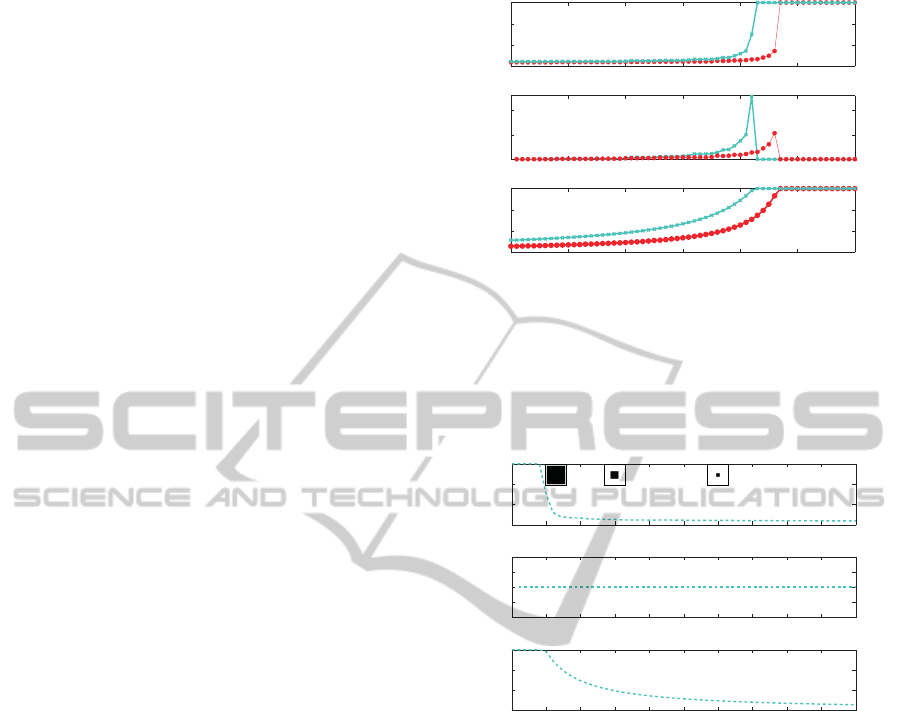
Figure 1: Responses to approaching looming stimulus at
2m/s, with different sizes. Dotted red line: results from the
10 × 10 pixels object size; Crossed blue line: results from
the 20 × 20 pixels object size. Top graphs: slope of the
averaged power spectra α, computed for each time instant.
Middle graphs: slope variation across time (∆α). Bottom
graphs: angular size as the object approaches to the camera,
reaching a final angular size of 60 degrees (equation 6).
0 0.05 0.1 0.15 0.2 0.25 0.3 0.35 0.4 0.45 0.5
−3
−2
−1
0
Slope of the averaged
Power spectra
0 0.05 0.1 0.15 0.2 0.25 0.3 0.35 0.4 0.45 0.5
0
20
40
60
Time to collision (seconds)
Angular size (deg)
0 0.05 0.1 0.15 0.2 0.25 0.3 0.35 0.4 0.45 0.5
−1
−0.5
0
0.5
1
Slope derivative
(α)
(Δα)
Figure 2: Responses to a receding stimulus at 2m/s, with
10 × 10 pixels of size. The legend is similar to figure 1.
In top pannel, it is depicted three different frames of the
receding object, captured at the time instant indicated on
the x−axis.
well as its variation (∆α) follows the increment on the
angular size of the visual stimuli, taking higher val-
ues as the object approaches the camera, ∆α peaking
when the angular size of the approaching objects was,
approximately, 56 degrees. Adittionally, ∆α peak
value obtained is higher for the biggest object sim-
ulated (∆α
peak
≃1.28 for object size of 10 ×10 pixels
and 0.53 for 20 × 20 pixels).
In order to verify if ∆α value is a good indicator
of the trajectory or proximity of the object, a receding
trajectory, for an object of 10 × 10 pixels was gener-
ated.
Comparing the results obtained for approaching
(figure 1) and receding objects (figure 2), significant
differences can be observed, both on the top and mid-
dle graphs (indicating the slope of the average power
spectra and the slope variation for each time instant,
ATime-analysisoftheSpatialPowerSpectraIndicatestheProximityandComplexityoftheSurroundingEnvironment
151
0 0.1 0.2 0.3 0.4 0.5 0.6 0.7 0.8 0.9 1
−2.85
−2.8
−2.75
−2.7
Slope of the averaged
Power spectra
0 0.1 0.2 0.3 0.4 0.5 0.6 0.7 0.8 0.9 1
4
6
8
10
12
Time (seconds)
Angular size (deg)
0 0.1 0.2 0.3 0.4 0.5 0.6 0.7 0.8 0.9 1
0
0.02
0.04
0.06
Slope derivative
(α)
(Δα)
Figure 3: Responses to stimulus translating at 1m/s, with
different sizes. This legend is similar to the one from figure
1.
respectively). α value tends to increase as the ob-
ject approaches, being an indicator of the object prox-
imity. On the other hand, for the receding situation
tested, α value tends to decrease, directly following
the object angular size decrement.
Additionally, a translatory trajectory was created,
for the same object sizes used in the case of the
approaching trajectory. The simulated objects per-
formed a translational trajectory at 1 meter to the cam-
era, moving at a speed of 1m/s. The obtained results
can be observed on figure 3.
According to the results obtained for two objects,
with distinct sizes, translating at 1m/s and comparing
them to the previous results (figure 1 and 2), we ver-
ify that both α and △α are much more constant across
all the video sequence time, being, the hindmost, sub-
stantially lower than the ∆α values obtained for the
previous situations tested.
In a robotic perspective, by applying a mere
threshold mechanism to the output of the slope vari-
ation graph, a simple collision avoidance artificial
mechanism could be developed.
In order to analyse the variation of both param-
eters (α and ∆α) in more realistic visual scenarios,
shaddow effects, as well as a 3D perspective view was
added to the simulated video sequence. The video se-
quence generated has 320 × 180 pixels in size, and a
sampling rate of 30 frames/s. Two approaching or-
ange balls were introduced in the green visual scene,
both with 5 cm, and approaching at 0.36 m/s, approx-
imately.
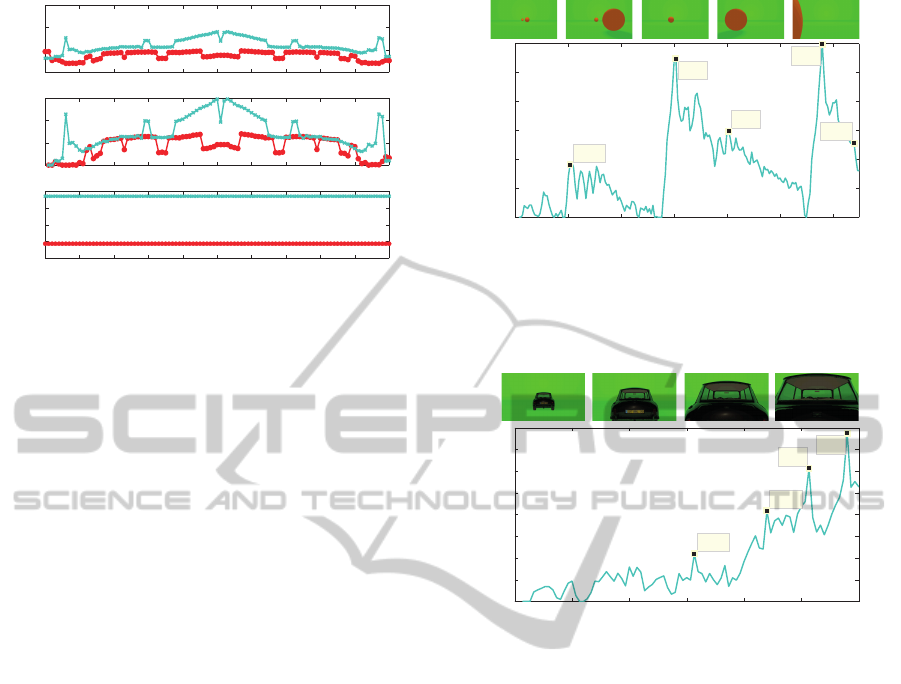
Figure 4 shows the ∆α value obtained for each
frame of the image sequence previously described.
Important time instants were highlighted in the slope
derivative graph. The first bigger ∆α peak was pro-
duced at t =3.003 s, signalling the moment when of
the the approaching ball was very close to the camera
(second video frame, on figure 4). Then, ∆α started
(Δα)
0 1 2 3 4 5 6
0
0.02
0.04
0.06
0.08
0.1
0.12
X: 3.033
Y: 0.1097
Time (seconds)
Slope derivative
X: 5.8
Y: 0.1195
X: 6.4
Y: 0.05111
X: 1.033
Y: 0.03625
X: 4.033
Y: 0.0595
Figure 4: Slope variation (∆α) obtained for each frame of
the image sequence previously described. Five important
time instants are pointed out on the graph, and the video
frames corresponding to those time instants are sequentially
disposed on the image top.
(Δα)
0 0.5 1 1.5 2 2.5 3
0
0.02
0.04
0.06
0.08
0.1
0.12
0.14
0.16
X: 1.567
Y: 0.04378
Time (seconds)
Slope derivative
X: 2.2
Y: 0.08334
X: 2.567
Y: 0.1225
X: 2.9
Y: 0.1548
Figure 5: Slope variation (∆α) obtained for the images cap-
tured by a camera approaching a car. Four important time
instants are pointed out on the graph, and the video frames
corresponding to those time instants are sequentially dis-
posed on the image top.
to decrease, being an indicator of the distant location
where the second ball was located. At t = 5.8 s, a
second ∆α peak was achieved, signalling the moment
when the second ball was close by. After that point
in time, the ∆α started to decrease because the ap-
proaching ball become, only partially, within the cap-
tured image. Based on these results obtained so far,
we verified that, the △α value is a good indicator of
the proximity of the objects in the visual scene, even
when this is composed by multiple objects.
In the last simulation tested, two conditions were
modified: motion and complexity. In this case, the
camera is the one that moves on the environment, ap-
proaching a static car, which complexity, in terms of
shape and texture, is highly superior to the previous
situations tested (figure 5).
Figure 5 shows, that even changing movement and
complexity conditions, the increment on the ∆α value
follows the approximation of the camera in relation to
the stationary car.
ICINCO2014-11thInternationalConferenceonInformaticsinControl,AutomationandRobotics
152
4.2 Real Image Sequences
4.2.1 Real Image Sequence, Showing a Dynamic
Complex Environment
In order to analyse the changes in the slope of the
power spectra (∆α) for real images, a real video
sequence with a PlayStation eye camera was cap-
tured. Along the recording time, we kept changing
the environment, adding new objects to the area being
recorded, as well as moving the objects closer or de-
viating away from the camera. Images selected from
the video sequence recorded are represented on figure
6.
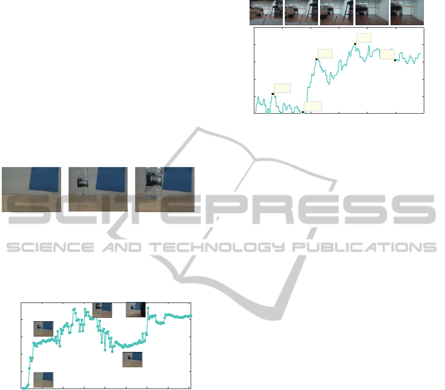
A B
C
Figure 6: Images selected from the video sequence, show-
ing: A: simple environment; B: the introduction of an empty
bootle; C: the approaching of the bottle to the camera.
After computing ∆α values for each frame of the
captured video, the following graph was obtained (fig-
ure 7).
0 2 4 6 8 10 12 14 16
0
0.05
0.1
0.15
0.2
0.25
Time (seconds)
Slope derivative
A
B
C
D
E
(Δα)
Figure 7: Slope variation (∆α) obtained for the images cap-
tured by a camera, for a complex and dynamic real environ-
ment. Five important time instants are signed on the graph
(A-E), and the video frames corresponding to those time in-
stants are placed close to the signalling letters.
Analyzing the graph on figure 7, and taking into
account the images selected from the video record-
ing, we see that, in A, the visual scenario is quite sim-
ple, which leads to a lower ∆α value. In B, a new
object was added to the arena, which led to an ac-
centuated slope increment. Then, we started slowly
approching the water bottle to the camera, which led
to a slowly increase in ∆α (C). Then, the water bottle
started to recede in relation to the camera, leading to
a slowly ∆α decrease (D). Finally, in E, a new object
was added to the recorded arena, which led to a ∆α
value increment.
This experiment proves the efficiency of the
methodology here proposed when implemented in a
0 2 4 6 8 10 12
0
0.05
0.1
0.15
0.2
0.25
X: 1.337
Y: 0.05637
Time (seconds)
Slope derivative
X: 3.442
Y: 0.003883
X: 4.411
Y: 0.1575
X: 7.151
Y: 0.2024
X: 9.958
Y: 0.1548
(Δα)
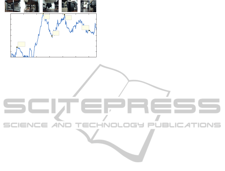
Figure 8: Slope variation (∆α) obtained for the images cap-
tured by a camera placed on a Pionner robot, moving for-
ward in a real lab environment. In the top of the graph,
selected frames are disposed sequentially - black arrow in-
dicates future robot positions.
real environment. By analysing the ∆α variations
across time, we can infer about the complexity of the
environment, as well as about the proximity of the ob-
jects in relation to the camera.
4.2.2 Experimental Results using a Pioneer 3DX
Robot
In order to test the methodology in real time and in-
side a lab environment, a real robot, the Pioneer 3-
DX, was used. A PlayStation Eye digital camera was
used to obtain the video segments.
In the first situation tested, the Pioneer robot was
moving forward at, approximatly, 13 cm/s in a non-
structured lab environment. Images captured by the
camera were resized online to a smaller size (160 ×
120 pixels) in order to decrease the processing time
required.
Figure 8 shows the results obtained for the men-
tioned situation.
Similarly to the results depicted on figure 7, ∆α
values obtained for this video sequence (figure 8) are
a good indicator of the surrounding environment com-
plexity, as well about the objects proximity to the
camera - and, indirectly, to the robot. Along the time
interval between 0 and 4 seconds, ∆α value is kept
low (below 0.06), presenting some minor amplitude
variations, due to the fact that, in the beginning, the
camera on the robot was not completely stable, show-
ing some small drifts. At t = 4.411 s, ∆α highly in-
creases, indicating the proximity of the camera to the
chair and box located in diagonal to the robot trajec-
tory (top of figure 8, third frame). After that point in
time, when capturing a more open field, ∆α started to
decrease. However, due to the continous movement
of the robot, in direction to the walls of the lab, the
∆α restarted to increase (t = 7.151s). After that point,
and due to the big number of different objects located
ATime-analysisoftheSpatialPowerSpectraIndicatestheProximityandComplexityoftheSurroundingEnvironment
153
0 5 10 15 20 25 30
0
0.2
0.4
0.6
0.8
1
1.2
1.4
1.6
X: 12.5
Y: 1.59
Time (seconds)
Slope derivative
X: 2.5
Y: 0.3618
X: 20.7
Y: 1.557
X: 15.9
Y: 0.771
X: 30.3
Y: 0.9745
(Δα)
Figure 9: Slope variation (∆α) obtained for a video se-
quence captured during a 360 deg rotation of the Pioneer
robot, in a cluttered environment. In the top of the graph,
selected frames are disposed sequentially, corresponding to
the images of the datapoints highlighted in the graph.
in the front of the robot, some small variations were
verified in the ∆α values. Despite those variations, the
values were constantly high, reflecting the complex-
ity and proximity of the objects on the surrounding
environment.
Besides the forward movement of the robot, an
additional experiment was performed. In this second
situation, the robot was stationary, performing a com-
plete 360 degree rotation over its own axis, at a speed
of 11 deg/s. The main goal of this experimnt was to
verify if, different types of movement (translatory ver-
sus rotational) induce distinct results.
Figure 9 shows that ∆α values decreased for im-
ages showing, either a lower number of objects in the
robot vinicity - lower complexity - or when the objects
are located far away from the robot - indicating possi-
ble safer paths. (frames 3 and 5). However, when the
objects are nearer or when present in a big quantity
(frames 2 and 4) ∆α value increases.
According to these results, the method of calcu-
lating the ∆α value for real image sequences could be
useful to provide information about the complexity of
the environment, and even to help the robot to choose
a less complicated and safer route of escape.
5 CONCLUSIONS
In this paper we have adressed the detailed structure
of the temporal variation of the spatial power spec-
tra, computed for a high range of different image se-
quences. Distinct visual scenarios complexity and tra-
jectories were constructed - simulation - and recorded
- in a real environment. Based on the results obtained,
we concluded that the approach here proposed is very
general and is able to indicate the proximity and the
complexity of the vicinity.
Experiments with a Pioneer-3DX robot showed
that, this methodology is able to work in real time,
giving indication about possible “safer” paths to the
robot, when, for example, the robot is performing an
exploraty mission or trying to escape from a possible
hazard. In the future, the methodology here presented
can also be applied in different fields of research, as
car safety, exploratory mission, among others.
ACKNOWLEDGEMENTS
This work has been supported by FCT – Fundação
para a Ciência e Tecnologia within the Project Scope
PEst OE/EEI/UI0319/2014. Ana Silva is supported
by PhD Grant SFRH/BD/70396/2010.
REFERENCES
Balboa, R. M. and Grzywacz, N. M. (2003). Power spectra
and distribution of contrasts of natural images from
different habitats. Vision Research, 43(24):2527–
2537.
Buccigrossi, R. and Simoncelli, E. (1999). Image compres-
sion via joint statistical characterization in the wavelet
domain. Image Processing, IEEE Transactions on,
8(12):1688–1701.
Burton, G. J. and Moorhead, I. R. (1987). Color and
spatial structure in natural scenes. Applied Optics,
26(1):157–170.
Doi, E., Gauthier, J. L., Field, G. D., Shlens, J., Sher, A.,
Greschner, M., Machado, T. A., Jepson, L. H., Math-
ieson, K., Gunning, D. E., Litke, A. M., Paninski,
L., Chichilnisky, E. J., and Simoncelli, E. P. (2012).
Efficient coding of spatial information in the primate
retina. The Journal of Neuroscience, 32(46):16256–
16264.
Dong, D. W. and Atick, J. J. (1995). Statistics of natural
time-varying images. Network: Computation in Neu-
ral Systems, pages 345–358.
Dror, R. O., O’Carroll, D. C., and Laughlin, S. B. (2000).
The role of natural image statistics in biological mo-
tion estimation. In Lee, S.-W., Balthoff, H. H., and
Poggio, T., editors, Biologically Motivated Computer
Vision, volume 1811 of Lecture Notes in Computer
Science, pages 492–501. Springer Berlin Heidelberg.
Field, D. J. (1987). Relations between the statistics of natu-
ral images and the response properties of cortical cells.
J. Opt. Soc. Am. A, 4:2379–2394.
Field, D. J. and Brady, N. (1997). Visual sensitivity, blur
and the sources of variability in the amplitude spec-
tra of natural scenes. Vision Research, 37(23):3367 –
3383.
Hateren, J. (1992). A theory of maximizing sensory infor-
mation. Biological Cybernetics, 68(1):23–29.
Hateren, J. V. (1993). Spatiotemporal contrast sensitivity of
early vision. Vision Research, 33(2):257 – 267.
ICINCO2014-11thInternationalConferenceonInformaticsinControl,AutomationandRobotics
154

Hyvrinen, A., Hurri, J., and Hoyer, P. O. (2009). Natural
Image Statistics: A Probabilistic Approach to Early
Computational Vision. Springer Publishing Company,
Incorporated, 1st edition.
Liu, R., Li, Z., and Jia, J. (2008). Image partial blur detec-
tion and classification. Computer Vision and Pattern
Recognition, 2008. CVPR 2008. IEEE Conference on,
pages 1–8.
Nielsen, M. and Lillholm, M. (2001). What do features tell
about images? In Kerckhove, M., editor, Scale-Space
and Morphology in Computer Vision, volume 2106 of
Lecture Notes in Computer Science 2106, pages 39–
50. Springer Berlin Heidelberg.
Pouli, T., Cunningham, D. W., and Reinhard, E. (2010). Im-
age statistics and their applications in computer graph-
ics. Eurographics, State of the Art Report.
Rivait, D. and Langer, M. S. (2007). Spatiotemporal power
spectra of motion parallax: the case of cluttered 3d
scenes. In IS T-SPIE Symp. on El. Imaging.
Ruderman, D. L. (1997). Origins of scaling in natural im-
ages. Vision Research, 37:3385–3398.
Ruderman, D. L. and Bialek, W. (1994). Statistics of nat-
ural images: Scaling in the woods. Phys. Rev. Lett.,
73:814–817.
Simoncelli, E. P. and Olshausen, B. A. (2001). Natural
image statistics and neural representation. Annual
Review of Neuroscience, 24(1):1193–1216. PMID:
11520932.
Torralba, A. and Oliva, A. (2002). Depth estimation from
image structure. IEEE Transactions on Pattern Anal-
ysis and Machine Intelligence, 24:2002.
Wu, H., Zou, K., Zhang, T., Borst, A., and Kuhnlenz, K.
(2012). Insect-inspired high-speed motion vision sys-
tem for robot control. Biological Cybernetics, 106(8-
9):453–463.
ATime-analysisoftheSpatialPowerSpectraIndicatestheProximityandComplexityoftheSurroundingEnvironment
155
