
Numerical Simulation and Automatic Control of the pH Value in an
Industrial Blunting System
Vlad Mureşan
1
, Adrian Groza
2
, Mihail Abrudean
1
and Tiberiu Coloşi
1
1
Department of Automation, Technical University of Cluj-Napoca, Cluj-Napoca, Romania
2
Department of Computer Science, Technical University of Cluj-Napoca, Cluj-Napoca, Romania
Keywords: Distributed Parameter Process, Control System, Numerical Simulation Method, Matrix of Partial
Derivatives of the State Vector, Taylor Series, pH.
Abstract: A solution for the pH control of the residual water in an industrial blunting system is proposed. The
technological process associated to the blunting system is decomposed in four sub-processes connected in
series and in parallel, each of them being a distributed parameter one. The mathematical models of the sub-
processes are expressed using partial differential equations. Both this procedure and the advanced structure
of the control system generate very high control performances. For the numerical simulation of the control
system, a numerical method based on the Matrix of Partial Derivatives of the State Vector, associated with
Taylor series is proposed. This method permits the numerical simulation of the systems that include in their
structure distributed parameter processes. The conducted simulations proved high accuracy of our original
method.
1 INTRODUCTION
The blunting system treated in this paper belongs to
a metallurgical factory. Its purpose is to assure a
value of the pH of residual water around 7 at the
overflowing point. The pH control of the residual
water is necessary in order to avoid the pollution of
the closest river (in general the residual water is
overflowed in the closest river) (Moore, 1978). The
residual water has an acid character (pH < 7) and the
reacting substance used in order to neutralize the
acid is the cream of lime (with pH value 12).
The system contains four tanks in its structure,
with the same role and the same technical
characteristics, connected in series through some
orifices (Mureşan et al., 2012). The two reactants are
introduced in the chemical reaction at the edge of the
first tank, edge which does not communicate with
the second tank. The overflowing point from the
system is placed at the edge of the fourth tank, edge
which doesn’t communicate with the third tank. In
order to apply an advanced control structure (for
example the cascade one (Love, 2007)) the system is
decomposed in two subsystems, the first one being
associated to the first tank and the second one
including the last three tanks. The last three tanks
will be treated as an equivalent tank with the length
three times bigger than the length of the initial ones.
Both the technical characteristics of the tank number
1 associated to the first subsystem and of the
equivalent tank associated to second one, are
presented in the Table 1:
Table 1: The technical characteristics of the tanks.
The technical
characteristics of
the tank
The
length
The
width
The
depth
The
volume
Tank 1 5 m 2 m 1.5 m 15 m
3
The equivalent
Tank (Tank 2 +
Tank 3 + Tank 4)
15 m 2 m 1.5 m 45 m
3
The pH value of the residual water can be
controlled adjusting the flow of the cream of lime
that is introduced in the process (Vînătoru, 2001),
(Golnaraghi and Kuo, 2009). The control signals
generated by the pH controllers are unified current
ones (4-20 mA). The final control signal (unified
current signal) is applied to the actuator (an electro-
valve on the cream of lime pipe). The output signals
from the pH transducers (the feedback signals) are
unified current signals, too.
540
Mure¸san V., Groza A., Abrudean M. and Colo¸si T..
Numerical Simulation and Automatic Control of the pH Value in an Industrial Blunting System.
DOI: 10.5220/0005062505400549
In Proceedings of the 11th International Conference on Informatics in Control, Automation and Robotics (ICINCO-2014), pages 540-549
ISBN: 978-989-758-039-0
Copyright
c
2014 SCITEPRESS (Science and Technology Publications, Lda.)
2 MODELING THE
TECHNOLOGICAL PROCESS
AND THE AUTOMATIC
CONTROL SYSTEM
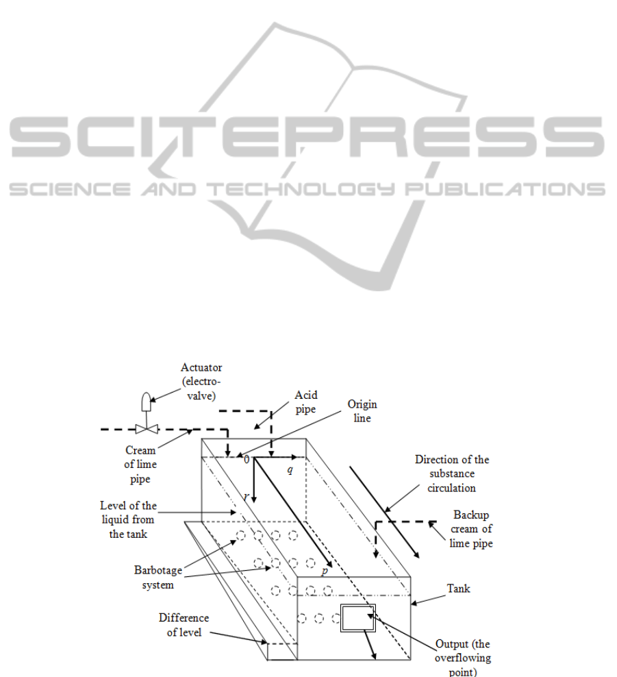
The general structure of both tank number 1 and
equivalent tank is presented in Fig. 1, without
considering, in this moment, the difference of length
between them. The two dashed lines near the origin
line are associated only to the first tank, respectively
the third dash line and the difference of level are
associated only to the equivalent tank. The
substances circulation from the input to the output
point of the tanks appears both due to the small level
differences between the consecutive tanks and due to
the barbotage mix-up systems from the tanks
structure. In this case, the chemical reaction occurs
progressively, the pH value depending both on time
and the position in the tanks. The conclusion is the
fact that the technological blunting processes
associated to the tanks are distributed parameter
ones.
In Fig. 1, the pH variation in relation to position
in the tanks volume (Li and Qi, 2011) is highlighted
through the axes of the Cartesian system. As it can
be remarked in Fig. 1, the origin of the Cartesian
system is the center of the origin line (in relation to
the tanks width) and the pH variation in relation to
the tanks length, width and depth corresponds with
the pH variation along the axes 0p, 0q, respectively
0r. Due to the efficient homogenization of the pH in
the tanks width and depth assured by the barbotage
system, the weight of the pH variation along the 0q
and 0r axes is insignificant in comparison with the
0p axis case. Hence, in the model of the processes
only the pH variation in the tanks length (on the 0p
axis) is considered.
The two technological processes associated to
the two tanks (tank 1 and the equivalent tank) can be
decomposed each in two sub-processes connected in
parallel. In each case, the sub-processes are
associated with the acid’s, respectively the cream of
lime’s effects and they are modeled considering the
indifferent pH value (7). The output signal from
each process results as the sum of the output signals
from the corresponding sub-processes. Also the
output signals from the sub-processes of the same
process have an antagonistic effect one in relation to
other, introducing the possibility of the pH control.
In Fig. 2, the proposed control structure is
presented. Due to the fact that the two processes are
connected in series and they contain each two sub-
processes connected in parallel, the whole blunting
process contains four sub-processes connected in
series and in parallel, as it can be remarked in Fig. 2.
Our solution is a combined control structure
cascade + feed-forward. The C elements are the
controllers (including CB – the compensation
block), the A element is the actuator (an electro-
valve on the cream of lime pipe) and K
pH
is a
constant equal to 5 (pH of cream of lime – 7). MT1,
MT2, and MT3 are pH transducers and MT4 is a
flow transducer. The significance of the signals
Figure 1: The general structure of the tanks from the blunting system.
NumericalSimulationandAutomaticControlofthepHValueinanIndustrialBluntingSystem
541
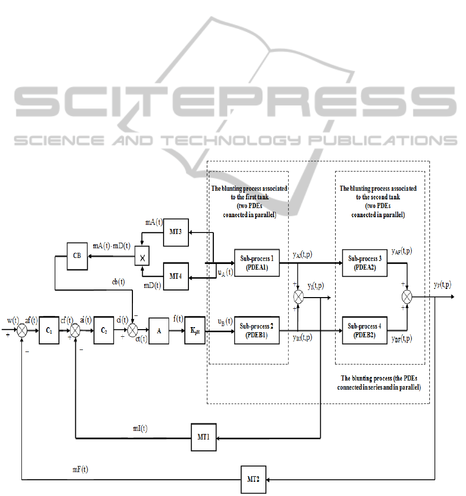
notations is: y – output signals of processes and sub-
processes, m – measurement signals, c – control
signals, w – the reference signal, a – error signal,
u – input signals in the process and f – actuating
signal (the flow of cream of lime). These general
notations are singularized in Fig. 2 for each element.
The input signals u are equal to the product between
the flow of the reactants and their pH. In the control
structure, the effect of the acid, propagated through
PDEA1 and PDEA2 (Fig. 2) is treated as a
disturbance.
The model of the distributed parameter sub-
processes from the structure of the blunting process
is expressed using partial differential equations
(PDEs in Fig. 2) (Krstic, 2006), (Curtain and Morris,
2009), (Smyshlyaev and Krstic, 2005). The control
effect is propagated at the process output through the
effect of the base (cream of lime), more exactly
through PDEB1 and PDEB2 elements. The reference
w is fixed at a value in unified current, proportional
with 7 (pH indifferent value). The equipment from
the control structure works in unified current.
The general form of the partial differential
equation that describes the working of each sub-
process from Fig. 2, is presented in relation 1.
a
00
· y
00
+ a
10
· y
10
+ a
01
· y
01
+ a
20
· y
20
+
+ a
11
· y
11
+a
02
· y
02
= φ
00
,
(1)
In relation (1), the notations y
....
= y
....
(t,p), φ
00
=
= φ
00
(t,p),
TP T P
TP
(y py/t)
+
, T=0,1,2…., and
P=0,1,2,.., are used and (t), respectively (p) are the
independent variables time and length. Also, in this
paper, only one numerical index attached to a signal
represents the differentiation order of that signal in
relation to the independent variable time (t).
Relation (1) can be singularized for each PDE
A1, A2, B1 and B2. In (1) the (a...) coefficients are
constant and depend as value on the values of the
time constants of the sub-processes and the values of
their “length constants”. The time constants are
identified using the tangent method applied on the
experimental curves. In the modeling procedure the
linear increasing of these constants along the 0p axis
is considered. The length constants are identified
using a method based on interpolation. y(t,p) (y
represents the pH value) and φ(t,p) functions respect
Figure 2: The proposed control structure.
ICINCO2014-11thInternationalConferenceonInformaticsinControl,AutomationandRobotics
542

the Cauchy continuity conditions. Relation (1) can
be rewritten so that in the right member remains
only the element y
20
, being obvious the fact that the
state variables are y
00
and y
10
. The other state
variables result from the equations that describe the
working of the other elements from the control
structure, these being lumped parameter ones (their
working depends only by (t) independent variable
and it can be modeled using ordinary differential
equations (ODE)) (Love, 2007), (Golnaraghi and
Kuo, 2009). All the transducers from the control
structure and the actuator are first order elements,
the controllers C
1
and C
2
are of PID type
(Proportional Integrator Derivative), respectively the
compensation block is of PD type. The modeling
procedure starts from the system of equations that
describe, in transitory regime, the working of each
element form Fig. 2. The system of equations is
following presented:
Transducer 1 (MT1):
I0
I1 T I00 I0
T
m
1
m [K y m ].
T
(2)
Transducer 2 (MT2):
F0
F1 T F0 0 F0
T
m
1
m [K y m ].
T
(3)
Transducer 3 (MT3):
A0
A1 T A0 A0
T
m
1
m [K A m ].
T
(4)
Transducer 4 (MT4):
D0
D1 TD A0 D0
TD
m
1
m [K D m ].
T
(5)
PID controller 1 (C1):
0
1P
C
cf
1
cf [K
T
C1 0 F0 DC1 1 F1 0
2 PC1 1 F1 IC1 0 F0
C
(w m ) K (w m ) cf ]
1
cf [K (w m ) K (w m ) . (6)
T
DC1 2 F2 1
K (w m ) cf ]
PID controller 2 (C2):
0
1PC2
C
ci
1
ci [K
T
0I0 DC21I1 0
2 PC2 1 I1 IC2 0 I0
C
(cf m ) K (cf m ) ci ]
1
ci [K (cf m ) K (cf m ) . (7)
T
DC2 2 I 2 1
K (cf m ) ci ]
Actuator (A):
B0
pH
B1 A 0 B0
A
u
1
u(KKctu).
T
(8)
Compensation block (CB)
0
1
CB
cb
1
cb [
T
PCB 0 0
DCB 0 0 0
2PCB00
CB
K (mD mA )
d
K ( (mD mA )) cb ]
dt
1d
cb [K ( (mD mA )) .
Tdt
2
DCB 0 0 1
2
(9)
d
K ( (mD mA )) cb ]
dt
The final control signal:
000
ct ci cb
(10)
Sub-processes 1-4 (i
{AI,AF,BI,BF}) (PDE
II·2):
i00
i10
i20 i00 00 i00 10 i10
20
01 i01 11 i11 02 i02
y
y
1
y[(ayay
a
ay ay ay)]
(11)
The output signal from the process associated to
the first tank:
I0 AI0 BI0
yy y
(12)
The output signal from the process associated to
the second tank:
F0 AF0 BF0
yy y
(13)
Relation (11) results from relation (1) rewritten
in the presented form. Using the equations
associated to these elements and relation (1)
singularized for the four sub-processes, two state
vectors result. The first state vector is associated to
the main control system from Fig. 2 and results from
NumericalSimulationandAutomaticControlofthepHValueinanIndustrialBluntingSystem
543
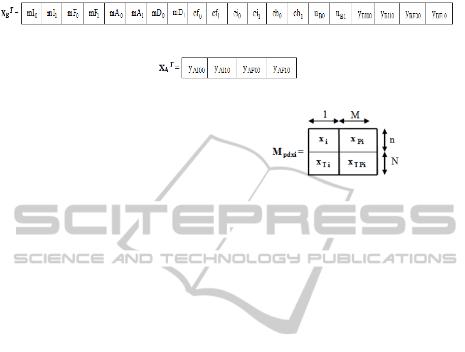
Figure 3: The state vector associated to the main control signal.
Figure 4: The state vector associated to the propagation of the acid effect.
relations (2), (3), (4), (5), (6), (7), (8), (9),
respectively (11) (for i
{BI,BF}). The first state
vector contains 20 elements. The second one is
associated to the disturbance propagation effect,
containing 4 elements (the y
00
and y
10
elements
associated to PDEA1 and PDEA2 from relation
(11)). The two state vectors, in transposed form, are
presented in Fig. 3 and Fig. 4. The significance of
the new notations used in relations (2) – (13) is:
T
K
– proportionality constant of the pH transducers;
T
T
– time constant of the pH transducers;
TD
K –
proportionality constant of the flow transducer;
TD
T
– time constant of the flow transducer;
A0
A – pH
value of the acid at the input in the tank;
A0
D – acid
flow at the input in the tank;
C
T – time constant of
the two controllers C
1
and C
2
;
PC1
K and
PC2
K –
proportionality constants of the two controllers C
1
and C
2
;
IC1
K and
IC2
K – – integral constants
of the two controllers C
1
and C
2
;
DC1
K and
DC2
K
– derivative constants of the two controllers C
1
and
C
2
;
A
T – time constant of the actuator;
A
K –
proportionality constant of the actuator;
pH
K
–
proportionality constant equal to 5 (the difference
between the cream of lime pH and the indifferent pH
value (7));
CB
T – time constant of the compensation
block;
PCB
K – proportionality constant of the
compensation block;
DCB
K – – derivative
constant of the compensation block.
In order to simulate the control structure that
includes 4 PDEs (that involve major simulation
problems) on the computer and using the state
vectors, the two Matrices of Partial Derivatives of
the State Vector (Mpdx) (Coloşi et al., 2013) can be
determined, with the general form presented in
relation (14).
In (14) the significance of the notations is: x –
– the state vector, x
Ti
– the vector of partial
derivatives of the state vector in relation to time (t)
(the first elements of the x
Ti
vector are the pivot
elements), x
Pi
– the matrix of partial derivatives of
(14)
the state vector in relation to length (p), x
TPi
– the
matrix of partial derivatives of the state vector in
relation both to time (t) and length (p). Also the
index i signifies that relation (14) can be
singularized for the two previous mentioned cases.
The (Mpdx) associated to the control system has the
dimension (70×9) (M = 8; n = 20; N = 50). Morever,
the (Mpdx) associated to the propagation of the acid
effect has the dimension (14×9) (M = 8; n = 4;
N = 10). For the initialization of the matrices from
(14), the analytical approximating solution that
verifies (1) can be used, solution that is a product of
exponential functions. In the case of PDEA1 and
PDEA2, the analytical approximating solution has a
decreasing evolution both in relation to (t) and (p).
Differently, in the case of PDEB1 and PDEB2, the
solution has an increasing evolution in relation with
both independent variables. After the initialization,
the numerical simulation algorithm can start. To
advance from the sequence (k) to the next one (k+1)
the Taylor series are used, resulting the elements of
the x vector and of the x
Pi
matrix. Using these
values, the elements of the x
Ti
vector and of the x
TPi
matrix. The algorithm stops at the predefined period
of time and the integration step is considered small
enough for a correct numerical integration.
3 THE SIMULATIONS RESULTS
The simulations are made in MATLAB.
The imposed performances to the control
structure are: steady state error at position equal to 0,
overshoot smaller, in module, than 2.5%, settling
time smaller than 20 min, respectively the actuating
signal not to increase over the saturation limit. Also
one of the purposes of this paper is to determine the
control structure that generates the best set of
ICINCO2014-11thInternationalConferenceonInformaticsinControl,AutomationandRobotics
544

performances.
The two feedback signals associated to the
cascade structure result measuring the pH values at
the output of the two processes (at the output of tank
1, respectively equivalent tank). The process
associated to tank 1, due to the smaller length of this
tank, is faster than the process associated to
equivalent tank and it is included in the internal
loop. The compensation block CB (see Fig. 2)
receives the measurement signals of the flow and of
the pH value of the disturbance (of the acid
introduced in the reaction) and generates a control
signal that is finally subtracted from the control
signal C
2
. The compensation generated by CB
represents the feed-forward component of the
structure. The tuning of both controllers C
1
and C
2
is
made using an adapted form of module criterion for
the case when the model of the process is expressed
through PDEs (for this type of processes do not exist
specific tuning methods). Using the module criterion
(applied for second order processes) is obtained the
general form of the controller parameters, valid for
both controllers:
12
PC
EX
TT
K
2K T
,
IC
EX
K
2K T
1
,
12
DC
EX
TT
K
2K T
, where
1
T and
2
T (through singularization) are the time
constants corresponding to each of the two processes
(these constants are calculated in each of the two
cases for the corresponding values of (p)). Also,
T
AC
TTTT
. The
EX
K constant is present
in all three formulae and, while changing its value,
the three controller parameters are simultaneously
modified. Firstly, the value of the
EX
K is fixed for
the controller from the internal loop. After that,
another value of the
EX
K constant is chosen for the
controller from the external loop. The numerical
simulation of the control structure is made in order
to obtain the system performances. If the
performances are not enclosed in the imposed limits,
the value of
EX
K associated to C
1
is decreased
progressively, for each decrease the simulation of
the structure being repeated and, in each case the
obtained performances being evaluated. Hence, the
tuning method is an iterative one. In the case when,
from a simulation to the following one, the
performances of the system do not have a significant
improvement, the
EX
K constant associated to C
2
is
decreased as value and keeping this value constant,
the iterative procedure previously presented is
repeated (modifying only the parameters of C
1
) until
the imposed performances are obtained. In order to
obtain much better performances than the imposed
ones, the iterative tuning procedure can be
continued, but taking into consideration the variation
form and limits of the actuating signal. The variation
of the
EX
K constants between two successive
iterations, in both controller cases, has not an
imposed value (being modified considering the
grade of the performances improvement from an
iteration to the next one). In each controller case,
decreasing the value of the
EX
K constant we can
obtain a stronger control effect (action).
After obtaining the parameters of C
1
and C
2
, the
tuning of CB can be made. Using the same general
formulae, as in the case of C
1
and C
2
, but only a PD
structure, the
EX
K constant is decreased
progressively until the best possible performances
are obtained. After applying the presented
procedure, the following parameters are obtained:
for C
1
:
EX1
K 437.93 , for C
2
:
EX2
K0.35 ,
respectively for CB:
EXCB
K10 .
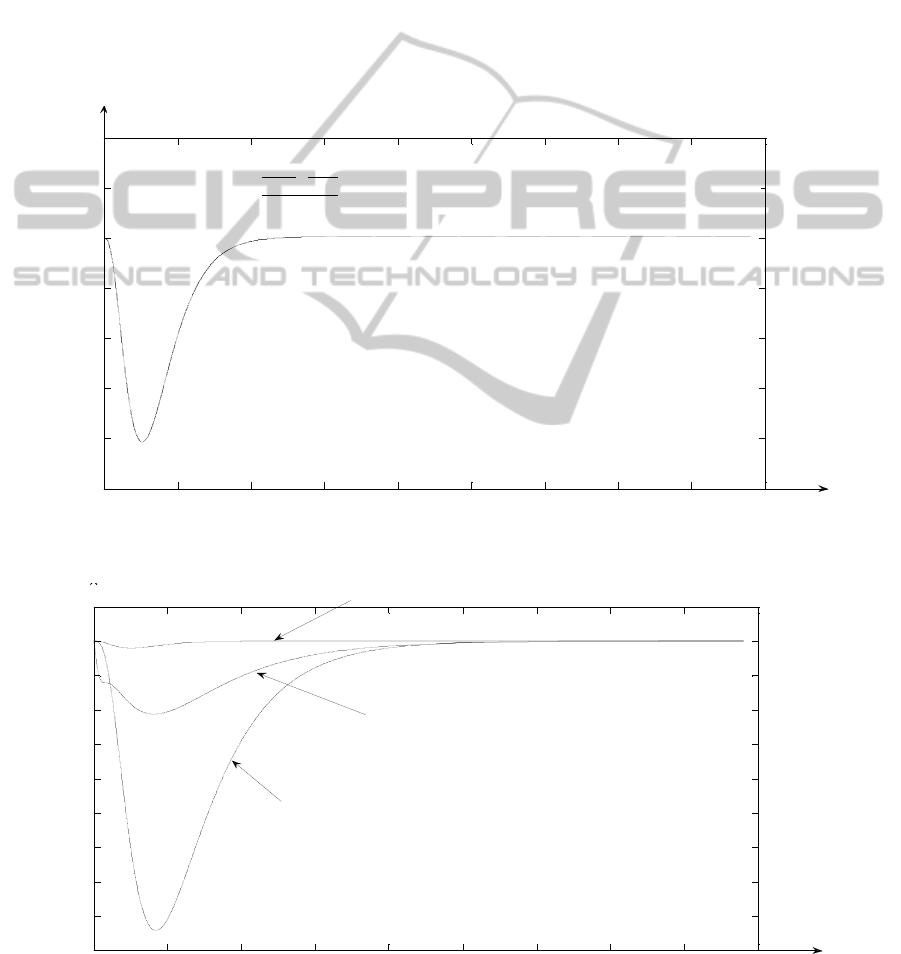
In Fig. 5, the comparative graph between the
automatic system’s analytical and numerical step
response is presented, at the overflowing point from
the system (the overflowing point of the equivalent
tank), considering the components of the disturbance
constants at the values pH
A
= 3 and D
A
(t) = 3l/s
(step disturbance, usual in the treated case).
On the graph the two responses cannot be
differentiated with the free eye due to the very small
errors between them. In steady state regime, the
value of cumulated relative error in percents
(Ungureşan and Niac, 2011) is proportional to
10
-3
%, this value very close to 0 showing the very
good numerical simulation performances. Also the
obtained control performances are very high ones,
the steady state error at position being 0 (the effect
of the disturbance is rejected), the settling time can
be considered 0 min because the value of the
response is enclosed in the stationary band of ±1%
around the steady state value (7) and the overshoot
module has an insignificant value of 0.03 % (the pH
variation around 7 does not affect the good working
of the system).
The necessity of using a very complex control
structure appears due to the fact that the imposed
performances to the control structure are very
restrictive ones, due to the sensitive character of the
application. In order to study the possibility of
NumericalSimulationandAutomaticControlofthepHValueinanIndustrialBluntingSystem
545
reducing the cost of the control system, the structure
for Fig. 2 can be singularized to a simple cascade
structure or a simple feed-forward one. The
comparative graph between the responses of the
three structures, in the same simulation conditions as
in Fig. 5 case and for the controllers that generate
the best results that could be obtained is shown in
Fig. 6. For the case of cascade structure the
proportionality constant of the element CB is
considered 0. For the feed-forward structure, the C
2
equivalent value is considered 1 and the
proportionality constant of the MT element is
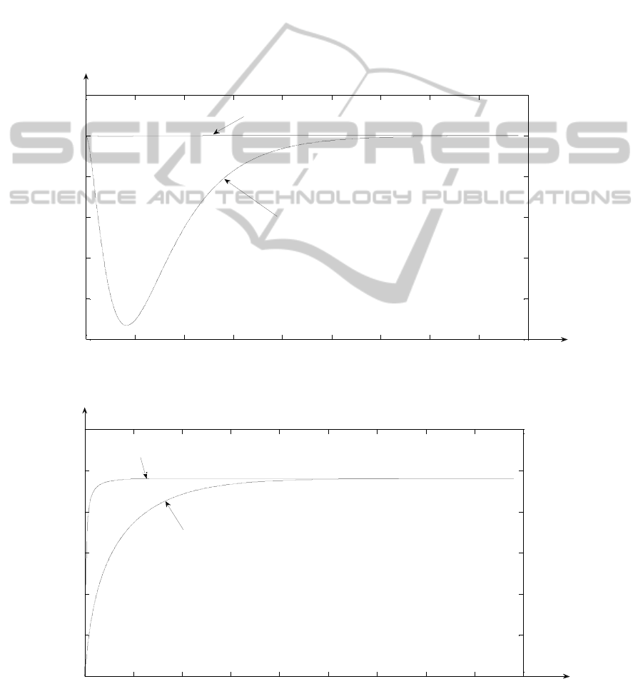
considered 0. It can be remarked from Fig. 6 that the
performances of the system decrease significantly if
we reduce the complexity of the control structure,
but, for this value of the disturbance, the simple
cascade or feed-forward structure can be used, too.
Also the using of a simple monocontour structure
(in Fig. 2 the compensation and the internal loops
will not appear and C
2
is made 1) is not an option
because it generates, in the best case an overshoot
with a value in module 7%, that is not functionally
permitted. This phenomenon is highlighted in Fig. 7
where the comparative graph between the system’s
numerical responses in the case of using a simple
feedback (monoconture) structure, respectively in
the case of using the advanced control structure
proposed in this paper, is presented.
Figure 5: Analytical and numerical step response of the system at the overflowing point.
Figure 6: Comparative graph between the simulations of different control structures.
0 20 40 60 80 100 120 140 160 180
6.9975
6.998
6.9985
6.999
6.9995
7
7.0005
TIME [min]
pH VALUE
The analytical response
The numerical response
0 20 40 60 80 100 120 140 160 180
6.91
6.92
6.93
6.94
6.95
6.96
6.97
6.98
6.99
7
7.01
TIME [min]
pH VALUE
The case of the simple cascade structure
The case of the simple feed-forward structure
The case of the combined structure (cascade+feed-forward)
ICINCO2014-11thInternationalConferenceonInformaticsinControl,AutomationandRobotics
546
The simulation from Fig. 6 is made for the best
controller that could be obtained for the simple
feedback control structure (
PR
K 8.2286
,
1
IR
K 0.4675 min
and
DR
K 34.7575 min
).
Another major disadvantage in using the simple
feedback control structure is an unacceptable value
of the response settling time, in this case 64 min.
In Fig. 8, the evolutions in time of the actuating
signals corresponding to the responses from Fig. 7,
are presented. From Fig. 8, it can be remarked that
the two actuating signals do not present value
“jumps”, respectively their maximum value (2.4 l/s)
is smaller than the saturation limit (4 l/s). The main
advantage of using the advanced control structure is
the fact that, due to the effect generated by the two
controllers and by the compensation block, the
corresponding actuating signal increases much faster
than in the case of using the simple control structure.
Practically, the three control elements force the rapid
increasing of the value of the actuating signal.
The control performances obtained in the case of
the four studied control structures are summarized in
Table 2. From Table 2 it obviously results that the
complex control structure from Fig. 2 generates the
best performances. Also, it results that, from the
other three (more simple) treated control structures,
the feed-forward type one generates good results.
Figure 7: Comparative graph between the responses of the advanced control system and of the simple feedback system.
Figure 8: The actuating signals.
0 20 40 60 80 100 120 140 160 180
6.5
6.6
6.7
6.8
6.9
7
7.1
TIME [min]
pH VALUE
The case of the combined control structure (cascade+feed-forward)
The case of the simple feedback control structure
0 20 40 60 80 100 120 140 160 180
0
0.5
1
1.5
2
2.5
3
TIME [min]
ACTUATING SIGNAL [l/s]
The case of the simple feedback control structure
The case of the combined control structure (cascade + feed-forward)
NumericalSimulationandAutomaticControlofthepHValueinanIndustrialBluntingSystem
547
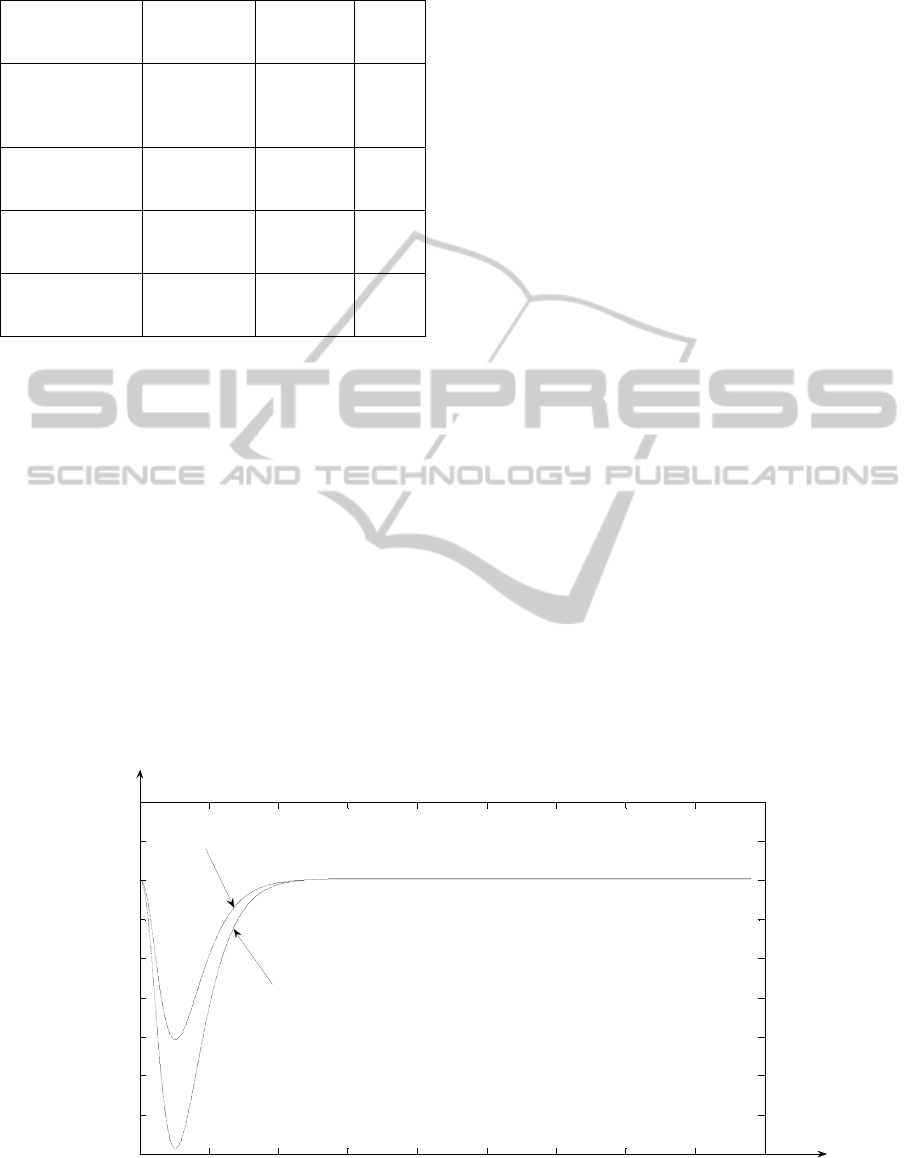
Table 2: The obtained performances.
Control
structure
Steady state
error at
position
Overshoot
(in
module)
Settlin
g time
The combined
structure
(cascade + feed-
forward)
0 0.03 %
≈0
min
The simple
cascade
structure
0 1.21 %
24
min
The simple
feed-forward
structure
0 0.28 %
≈0
min
The simple
feedback
control structure
0 7%
64
min
From the other simulations, it resulted that the
initial structure (Fig. 2) can efficiently reject the
effect of other types of disturbances, for example
sine type disturbances. In Fig. 9, the effect of a more
severe disturbance (pH
A
= 2 and D
A
(t) = 4 l/s) that
occurs in the process is presented. In this case, too,
the controllers, respectively the compensation block
reject very efficient the effect of the disturbance, the
obtained performances being comparable with the
case of the initial disturbance. The corresponding
actuating signal does not increase over the saturation
value, neither in this case.
4 CONCLUSIONS
We argue that the advanced control strategy
proposed in this paper (Fig. 2) assures good
performance (justified by Fig. 5-9).
The very high obtained control performances
prove that the advanced control strategy proposed by
the author in Fig. 2 is justified, the blunting process
being very restrictive from the ecological point of
view.
The fact that the process is viewed as a
distributed parameter one offers an important
technological advantage because the user has the
possibility to control the pH value in each point from
the tanks.
The original numerical simulation procedure
based on Mpdx and Taylor series, proposed in this
paper, generates a very high accuracy of the
simulation and offers the possibility to simulate
systems that include distributed parameter processes.
The simulations were made to test the system
before its physical implementation. In all the
simulation the value of the actuating signal does not
exceed the saturation limit.
In the presented approach, the effect of the acid
propagation phenomenon in the system is treated as
a disturbance. In this case, the value of the
disturbance is given by two components: the acid pH
and the acid flow at the input in the system.
The control system offers high performances even in
the case when a more severe disturbance occurs in
the process.
The main contributions of the authors in
elaborating this paper are: the process modeling
using partial differential equations; the
decomposition of the main process in four sub-
processes connected in series and in parallel; the
Figure 9: The effect of a more severe disturbance.
0 20 40 60 80 100 120 140 160 180
6.9965
6.997
6.9975
6.998
6.9985
6.999
6.9995
7
7.0005
7.001
TIME [min]
pH VALUE
The case with the initial disturbance
The case with a more severe disturbance
ICINCO2014-11thInternationalConferenceonInformaticsinControl,AutomationandRobotics
548

including of the four distributed parameter sub-
processes in a control structure; the usage of a
combined cascade + feed-forward control structure
for the pH control; the numerical simulation of the
proposed control structure using an original method
for the simulation of the distributed parameter
systems.
ACKNOWLEDGEMENTS
The research activity that helped the authors to
elaborate the paper was supported through the
research project “Green-Vanets”. The mentioned
research project is financed by the Technical
University of Cluj-Napoca.
REFERENCES
Coloşi, T., Abrudean, M., Ungureşan, M.-L., Mureşan, V.,
2013. Numerical Simulation of Distributed
Parameters Processes, Springer.
Curtain, R. F., Morris, K. A., 2009. Transfer Functions of
Distributed Parameter Systems, Automatica, 45, 5,
1101-1116.
Golnaraghi, F., Kuo, B. C., 2009. Automatic Control
Systems, Wiley.
Krstic, M., 2006. Systematization of approaches to
adaptive boundary control of PDEs. International J. of
Robust and Nonlinear Control, 16, 801-818.
Li, H.-X., Qi, C., 2011. Spatio-Temporal Modeling of
Nonlinear Distributed Parameter Systems: A
Time/Space Separation Based Approach, Springer, 1st
Edition.
Love, J., 2007. Process Automation Handbook, Springer,
1 edition.
Moore, R., 1978. Neutralization of waste water by pH
control, Instrument Society of America.
Mureşan, V., Abrudean, M., Ungureşan, M.-L., Coloşi, T.,
2012. Control of the Blunting Process of the Residual
Water from a Foundry. Proc. of IEEE SACI 7th
edition, Timisoara.
Smyshlyaev, A., Krstic, M., 2005. Control design for
PDEs with space-dependent diffusivity and time-
dependent reactivity, Automatica, 41, 1601-1608.
Ungureşan, M.-L., Niac, G., 2011. Pre-equilibrium
Kinetics. Modeling and Simulation. Russian J. of
Physical Chemistry, 85, 4, 549-556.
Vînătoru, M., 2001. Industrial plant automatic control,
Vol. 1, Universitaria Craiova.
NumericalSimulationandAutomaticControlofthepHValueinanIndustrialBluntingSystem
549
