
Real-time Local Stereo Matching
Using Edge Sensitive Adaptive Windows
Maarten Dumont, Patrik Goorts, Steven Maesen, Philippe Bekaert and Gauthier Lafruit
Hasselt University - tUL - iMinds, Expertise Centre for Digital Media, Wetenschapspark 2, 3590 Diepenbeek, Belgium
Keywords:
Stereo Matching, Adaptive Aggregation Windows, Real-time, Depth Estimation.
Abstract:
This paper presents a novel aggregation window method for stereo matching, by combining the disparity
hypothesis costs of multiple pixels in a local region more e fficiently for increased hypothesis confidence. We
propose two adaptive windows per pixel region, one following the horizontal edges in the image, the other
the vertical edges. Their combination defines the final aggregation window shape that rigorously follows all
object edges, yielding better disparity estimations with at least 0.5 dB gain over similar methods in literature,
especially around occluded areas. Also, a qualitative improvement is observed with smooth disparity maps,
respecting sharp object edges. Finally, these shape-adaptive aggregation windows are represented by a single
quadruple per pixel, thus supporting an efficient GPU implementation with negligible overhead.
1 INTRODUCTION
3D entertainment systems, like 3D gaming with ges-
ture recognition, 3DTV, etc. become increasingly
popular. Such systems often benefit from extracting
depth information by stereo matching instead of using
active depth sensing methods, which introduce factors
such as cost, indoor vs. outdoor lighting, sensitivity
range, etc.
To this end, we present a stereo matching algo-
rithm that provides improved disparity image quality
by exploiting not only the vertical edges in the image,
but also the horizontal edges, drastically improving its
robustness over a range of applications.
Stereo matching uses a pair of images to estimate
the apparent movement of the pixels from one image
to the next. This apparent movement is more specifi-
cally known as the parallax effect, as demonstrated in
Fig. 1, where two objects are shown, placed at differ-
ent depths in front of a stereo pair of cameras. When
moving from the left to the right camera view, an ob-
ject undergoes a displacement – called the disparity –
which is inversely proportional to the object’s depth in
the scene. Objects in the background (the palm tree)
will have a smaller disparity in comparison to objects
in the foreground (the blue buddy). The goal of stereo
matching is to compute a dense disparity map by es-
timating each pixel’s displacement.
There are typically 4 stages (Scharstein and
Szeliski, 2002) in local dense stereo matching: cost
Figure 1: Concept of stereo vision. A scene is captured
using 2 rectified cameras. Stereo matching attempts to
estimate the apparent movement of the objects across the
images. A large apparent movement (i.e. parallax) corre-
sponds to close objects (a low depth value) and vice versa.
calculation, cost aggregation, disparity selection, and
refinement. Our method follows these stages, which
is presented in an overview in Fig. 4.
First, we consider each disparity and we calcu-
late (in section 3) for each pixel in the left image the
difference between that pixel and the corresponding
pixel (based on the disparity under consideration) in
the right image.
Our main contribution can be found in the aggre-
gation step (in section 4), where the costs of neigh-
boring pixels are taken into account to acquire the
final cost. Previous methods typically use square
windows (Scharstein and Szeliski, 2002), where the
weight of each cost in the window can vary (Lu et al.,
2007b). Alternatively, variable window sizes are used
117
Dumont M., Goorts P., Maesen S., Bekaert P. and Lafruit G..
Real-time Local Stereo Matching Using Edge Sensitive Adaptive Windows.
DOI: 10.5220/0005065301170126
In Proceedings of the 11th International Conference on Signal Processing and Multimedia Applications (SIGMAP-2014), pages 117-126
ISBN: 978-989-758-046-8
Copyright
c
2014 SCITEPRESS (Science and Technology Publications, Lda.)
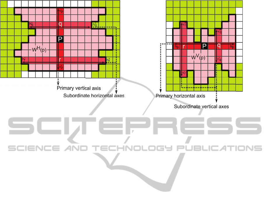
Figure 2: Derivation of the horizontal support window W
H
using each pixel’s axis-defining quadruple (h
−
p
, h
+
p
, v
−
p
, v
+
p
).
(Lu et al., 2007a), or the weights in the aggregation
windows are adapted to the images (Richardt et al.,
2010). In this paper, we use adaptive windows based
on the color values in the input images, as an exten-
sion to the method of (Zhang et al., 2009a). We create
two windows around the currently considered pixel,
based on the color information in the images (section
2). We assume that pixels with similar colors belong
to the same object, and therefore should get the same
disparity value. One window grows in the horizontal
direction and stops at edges; likewise the other win-
dow will grow in the vertical direction. Each win-
dow will favor a specific edge direction. Opposite to
the method of (Zhang et al., 2009a), which uses only
a horizontal window, we will combine these 2 direc-
tions, such that vertical edges are not favored.
Once the costs per pixel and per disparity are
known, the most suitable disparity with the lowest
cost is selected (in section 5) and the obtained dis-
parity map is intelligently refined in three stages (in
section 6).
Alternatively to local methods, global optimiza-
tion methods based on graph cuts (and similar)
(Yang et al., 2006; Wang et al., 2006; Papadakis
and Caselles, 2010), segmented patches (Zitnick and
Kang, 2007), and spatiotemporal consistency (Davis
et al., 2003) are used that do not necessarily follow
these steps.
To achieve high performance, we rely on par-
allel GPU computing by efficiently implementing
in CUDA, which exposes the GPU as a massive
SIMD architecture. Because of the specific nature of
the hardware, our method achieves real-time perfor-
mance. Results are presented in section 7, after which
we conclude in section 8.
Figure 3: Derivation of the vertical support window W
V
using each pixel’s axis-defining quadruple (h
−
p
, h
+
p
, v
−
p
, v
+
p
).
2 LOCAL SUPPORT WINDOWS
In the first step in our method, as shown in Fig. 4, we
determine a suitable support window W(p) for pixel
p of the left image I. This window is used to aggre-
gate the final cost for pixel p and should therefore be
chosen carefully. To construct the window for a pixel
p, we first determine a horizontal axis H(p) and ver-
tical axis V(p) crossing in p. These 2 axes can be
represented as a quadruple A(p):
A(p) = (h
−
p
, h
+
p
, v
−
p
, v
+
p
) (1)
where the component h
−
p
represents how many pixels
the horizontal axis extends on the left of p, v
+
p
repre-
sents how many pixels the vertical axis extends above
p, and so forth. This is shown in Fig. 2 and Fig. 3.
To determine each component using color consis-
tency, we keep extending an axis until the color dif-
ference between p and the outermost pixel q becomes
too large, i.e.
max
c∈
{
R,G,B
}
|
I
c
(p) − I
c
(q)
|
≤ τ (2)
where I
c
(p) is color channel c of pixel p, and τ is the
threshold for color consistency. We also stop extend-
ing if the size exceeds a maximum predefined size λ.
Using these 4 components, we define 2 local sup-
port windows for pixel p, referred to respectively as
the horizontal local support window W
H
(p) and the
vertical local support window W
V
(p).
Let’s start by defining the horizontal window
W
H
(p). First, we need to create its vertical axis based
on the values of v
−
p
and v
+
p
. We call this the primary
vertical axis V(p). Next, we consider the values of
SIGMAP2014-InternationalConferenceonSignalProcessingandMultimediaApplications
118
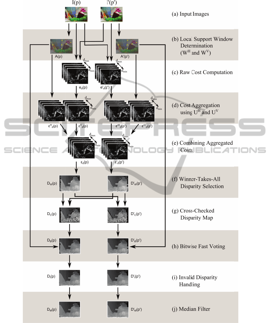
Figure 4: Overview of our method. (a) The input is a pair of rectified stereo images, in our case the standard Middlebury
dataset Teddy (Scharstein and Szeliski, 2003) (b) First, we calculate the local support windows, based on color similarities
in each image. (c) Next, we calculate the pixelwise cost per disparity. (d) These costs are aggregated, based on the support
windows. There are 2 windows, and therefore 2 sets of aggregated costs. (e) The costs of the 2 windows are combined. (f)
Next, we select the most suitable disparity value using a Winner-Takes-All approach. (g) A cross-check is performed to find
any mismatches, typically caused by occlusions around edges. (h) The local support windows are used again to determine
the most occurring disparity value in each window. This increases the quality of the disparity map. (i) Finally, any remaining
invalid disparities are handled and (j) a median filter is applied to remove noise. The result is 2 disparity maps, one for each
input image.
Real-timeLocalStereoMatchingUsingEdgeSensitiveAdaptive Windows
119

h
−
q
, and h
+
q
for each pixel q on the primary vertical
axis. These will define a horizontal axis per pixel q
on the primary vertical axis. These axes are called
the subordinate horizontal axes H (q). In short, this
results in the orthogonal decomposition:
W
H
(p) =
∪
q∈V(p)
H (q) (3)
An example is shown in Fig. 2.
Completely analogous but in the other direction,
we define the vertical local support window W
V
(p)
by creating a primary horizontal axis H(p) using h
−
p
,
and h
+
p
, and on this axis create the subordinate vertical
axes V (q):
W
V
(p) =
∪
q∈H(p)
V (q) (4)
An example is shown in Fig. 3.
The support windows W
H
(p) and W
V
(p) will
be used in the aggregation step, described in sec-
tion 4. By requiring only the single quadruple
(h
−
p
, h
+
p
, v
−
p
, v
+
p
) to define both windows, we reduce
memory usage, which is a serious consideration when
doing GPU computing.
Using this method to define aggregation windows,
we construct windows that are sensitive to edges in
the image. The horizontal window W
H
(p) will fold
nicely around vertical edges, because the width of
each subordinate horizontal axis is variable. Horizon-
tal edges are not followed as accurately, as the height
of the window is fixed and only determined by its
primary vertical axis. This situation, however, is re-
versed for W
V
(p). Thus by using both windows, we
do not favor a single edge direction, which will yield
better results.
Lastly, the notation W
′H
(p
′
) and W
′V
(p
′
) repre-
sents the local support windows for each pixel p
′
in
the right image I
′
.
3 PER-PIXEL MATCHING COST
For a disparity hypothesis d ∈ [d
min
, d
max
], consider
the raw per-pixel matching cost e
d
(p), defined as the
Sum of Absolute Differences (SAD):
e
d
(p) =
∑
c∈
{
R,G,B
}
|
I
c
(p) − I
′
c
(p
′
)
|
e
max
(5)
where p is a pixel in the left image I with correspond-
ing pixel p
′
in the right image I
′
, and the coordinates
of p = (x
p
, y
p
) and p
′
= (x
′
p
′
, y
′
p
′
) relate to the dispar-
ity hypothesis d as x
′
p
′
= x
p
− d, y
′
p
′
= y
p
.
The constant e
max
normalizes the cost e
d
(p) to the
floating point range [0, 1]. For example, when pro-
cessing RGB images with 8 bits per channel, e
max
=
3 × 255.
We calculate e
d
(p) for each pixel p and refer to it
as the per-pixel left confidence (or cost) map for dis-
parity d. Similarly the per-pixel right confidence map
can be constructed by calculating e
′
d
(p
′
) analogously
to Eq. 5, with the x-coordinates of p and p
′
now re-
lated as x
p
= x
′
p
′
+ d. The left and right per-pixel
confidence maps for disparity d = d
min
are shown in
Fig. 4(c).
4 COST AGGREGATION
For reliable cost aggregation, we symmetrically con-
sider both local support windows W (p) for pixel p in
the left image and W
′
(p
′
) for pixel p
′
in the right im-
age. If we only consider the local support window
W (p), the matching cost aggregation will be polluted
by outliers in the right image, and vice versa. There-
fore, while processing for disparity hypothesis d, the
two local support windows are combined into what
we will call a global support window U
d
(p). Dis-
tinguishing again between a horizontal and vertical
global support window, they are defined as:
U
H
d
(p) = W
H
(p) ∩W
′H
(p
′
) (6)
U
V
d
(p) = W
V
(p) ∩W
′V
(p
′
) (7)
where the coordinates of p = (x
p
, y
p
) and p
′
=
(x
′
p
′
, y
′
p
′
) are again related to the disparity hypothesis
d as x
′
p
′
= x
p
− d, y
′
p
′
= y
p
. In practice, this simplifies
beautifully to taking the component-wise minimum of
their axis quadruples from Eq. 1:
A
d
(p) = min
(
A(p), A
′
(p
′
)
)
(8)
Two – more confident – matching costs ε
H
d
(p) and
ε
V
d
(p) can now be aggregated over each pixel s of
the horizontal and vertical global support windows
U
H
d
(p) and U
V
d
(p) respectively:
ε
H
d
(p) =
1
U
H
d
(p)
∑
s∈U
H
d
(p)
e
d
(s) (9)
ε
V
d
(p) =
1
U
V
d
(p)
∑
s∈U
V
d
(p)
e
d
(s) (10)
where the number of pixels
∥
U
d
(p)
∥
in the support
window acts as a normalizer. These aggregated con-
fidence maps are shown in Fig. 4(d) for disparity hy-
pothesis d = d
min
.
SIGMAP2014-InternationalConferenceonSignalProcessingandMultimediaApplications
120

We next propose 2 methods to select the final ag-
gregated cost ε
d
(p), based on ε
H
d
(p) and ε
V
d
(p). The
first method takes the minimum and assumes that the
lowest cost will actually be the correct solution:
ε
d
(p) = min
(
ε
H
d
(p), ε
V
d
(p)
)
(11)
The second method uses a weighted sum and is
more robust against errors in the matching process:
ε
d
(p) = α ε
H
d
(p) + (1 −α) ε
V
d
(p) (12)
where α is a weighting parameter between 0 and 1.
Again this combined confidence map is shown in
Fig. 4(e).
The aggregation is repeated over the right im-
age, in order to arrive at a left and right aggregated
confidence map. This means computing A
′
d
(p
′
) =
min(A(p), A
′
(p
′
)), with p and p
′
now related as x
p
=
x
′
p
′
+d and from there setting up an analogous reason-
ing to end up at ε
′
d
(p
′
).
4.1 Fast Cost Aggregation Using
Orthogonal Integral Images
From the global axis quadruple A
d
(p) of Eq. 8 and
following the same reasoning that defined the local
support windows in section 2, an orthogonal decom-
position of the global support windows U
H
d
(p) and
U
V
d
(p) can be obtained, analogous to Eq. 3 and Eq. 4:
U
H
d
(p) =
∪
q∈V
d
(p)
H
d
(q) (13)
U
V
d
(p) =
∪
q∈H
d
(p)
V
d
(q) (14)
This orthogonal decomposition is key to a fast and
efficient implementation of the cost aggregation step.
Substituting Eq. 13 into Eq. 9 and Eq. 14 into Eq. 10,
we separate the inefficient
∑
s∈U
d
(p)
e
d
(s) into a hori-
zontal and vertical integration (Zhang et al., 2009a):
ε
H
d
(p) =
∑
q∈V
d
(p)
∑
s∈H
d
(q)
e
d
(s)
(15)
ε
V
d
(p) =
∑
q∈H
d
(p)
∑
s∈V
d
(q)
e
d
(s)
(16)
where the normalizer
1
∥
U
d
(p)
∥
has been omitted for
clarity.
For the global horizontal support window U
H
d
(p),
Eq. 15 intuitively means to first aggregate costs over
its subordinate horizontal axes H
d
(q) and then over
its primary vertical axis V
d
(p). Vice versa for the
vertical configuration of U
V
d
(p) in Eq. 16.
5 DISPARITY SELECTION
After the left and right aggregated confidence maps
from section 4 have been computed for every dis-
parity d ∈ [d
min
, d
max
], the best disparity per pixel
(i.e. the one with lowest cost ε
d
(p)) is selected using
a Winner-Takes-All approach:
D
W
(p) = argmin
d∈[d
min
,d
max
]
ε
d
(p) (17)
which results in the initial disparity maps D
W
(p) for
the left image and D
′
W
(p
′
) for the right image, both
shown in Fig. 4(f).
At the same time we also keep a final horizontally
and vertically aggregated confidence map:
ε
H
(p) = min
d∈[d
min
,d
max
]
ε
H
d
(p) (18)
ε
V
(p) = min
d∈[d
min
,d
max
]
ε
V
d
(p) (19)
Next we cross-check the disparities between the
two initial disparity maps for consistency. A left-
to-right cross-check of the left disparity map D
W
(p)
means that for each of its pixels p, the correspond-
ing pixel p
′
is determined in the right image based on
the disparity D
W
(p), and the disparity D
′
W
(p
′
) in the
right disparity map is compared to D
W
(p). If they dif-
fer, the cross-check fails and the disparity is marked
as invalid:
D
C
(p) =
{
D
W
(p) if D
W
(p) = D
′
W
(p
′
)
INVALID elsewhere
(20)
where p is now related to p
′
as x
′
p
′
= x
p
− D
W
(p),
y
′
p
′
= y
p
. The process is then reversed for a right-to-
left cross-check of the disparity map D
′
W
(p
′
), which
leaves us with the left and right cross-checked dispar-
ity maps D
C
(p) and D
′
C
(p
′
) to be refined in section
6.
Invalid disparities are most likely to occur around
edges in the image, where occlusions are present in
the scene. In Fig. 4(g) we show these occluded re-
gions as pure black (marked as invalid) pixels.
6 DISPARITY REFINEMENT
We refine the disparity maps found in the previous
section in three stages, (h) to (j) in Fig. 4.
First, the local support windows as described in
section 2 can be employed again, to update a pixel’s
disparity with the disparity that appears most inside
Real-timeLocalStereoMatchingUsingEdgeSensitiveAdaptive Windows
121

its windows. This method is the most powerful and is
detailed in section 6.1.
Next, any remaining invalid disparities are han-
dled in section 6.2.
Finally, the disparity map is filtered using a 3 × 3
median filter to remove any remaining speckle noise
in section 6.3.
6.1 Bitwise Fast Voting over Local
Support Windows
In this first stage of the refinement we will update a
pixel’s disparity with the disparity that is most present
inside its local support windows W
H
and W
V
as de-
fined in section 2. We may say that this refinement is
valid, because pixels in the same window have simi-
lar colors by definition, and therefore with high prob-
ability belong to the same object and should have the
same disparity. Confining the search to the local sup-
port windows also ensures that we greatly reduce the
risk of edge fattening artifacts.
To efficiently determine the most frequent dispar-
ity value within a support window, we apply a tech-
nique called Bitwise Fast Voting by (Zhang et al.,
2009b) and adapt it to handle both horizontally and
vertically oriented support windows. At the core of
the Bitwise Fast Voting technique lies a procedure that
derives each bit of the most frequent disparity inde-
pendently from the other bits. It is however reason-
able to assume this is valid (Zhang et al., 2009b).
First consider a pixel p with local support win-
dow W (p). We sum the lth bit b
l
(s) (either 0 or 1) of
the disparity value D
C
(s) of all pixels s in the support
window, and call the result B
l
(p). Furthermore distin-
guishing between horizontal and vertical support win-
dows, this gives:
B
H
l
(p) =
∑
s∈W
H
(p)
b
l
(s) (21)
B
V
l
(p) =
∑
s∈W
V
(p)
b
l
(s) (22)
The lth bit D
l
B
(p) of the final disparity value
D
B
(p) is then decided as:
D
l
B
(p) =
{
1 if B
l
(p) > β × N(p)
0 elsewhere
(23)
where β ∈ [0, 1] is a parameter that we will come back
to below.
This leaves us to determine exactly what B
l
(p)
and N(p) in Eq. 23 are. For this we again propose
two methods. The first method is similar to Eq. 11 and
relies on the minimum between the horizontally and
vertically aggregated confidence maps ε
H
(p) (Eq. 18)
and ε
V
(p) (Eq. 19):
B
l
(p) =
{
B
H
l
(p) if ε
H
(p) ≤ ε
V
(p)
B
V
l
(p) elsewhere
(24)
N(p) =
{
W
H
(p)
if ε
H
(p) ≤ ε
V
(p)
W
V
(p)
elsewhere
(25)
The second method uses a weighted sum:
B
l
(p) = α B
H
l
(p) + (1 −α) B
V
l
(p) (26)
N(p) = α
W
H
(p)
+ (1 −α)
W
V
(p)
(27)
where α is as in Eq. 12.
To recap, for a pixel p, Eq. 23 says that the lth bit
of its final disparity value is 1 if the lth bit appears as
1 in most of the disparity values under its local sup-
port window. The number of actual 1 appearances
are counted in B
l
(p), whereas the maximum possible
appearances of 1 is represented by the window size
N(p). The sensitivity parameter β controls how many
appearances of 1 are required to confidently vote the
result and is best set to 0.5.
It is important to note that certain disparities might
be invalid due to the cross-check of D
C
(p) in section
5. While counting bit votes, we must take this into
account by reducing N(p) accordingly. This way the
algorithm is able to update an invalid disparity by de-
pending on votes from valid neighbors, and thereby
reliably fill in occlusions and handle part of the im-
age borders. The improvement in quality that this
method yields in the disparity maps is already very
apparent from the visual difference between Fig. 4(f)
and Fig. 4(h).
A couple of key observations make that this
method is called fast. First, the number of iterations
needed to determine every bit of the final disparity
value is limited by d
max
. For example, in the Middle-
bury Teddy scene we use d
max
= 53, which represents
binary as 110101, and thus only 6 iterations suffice.
Furthermore, the votes can be counted very efficiently
by orthogonally separating Eq. 21 and Eq. 22, analo-
gously to Eq. 15 and Eq. 16. All this results in high
efficiency with low memory footprint.
6.2 Invalid Disparity Handling
The Bitwise Fast Voting technique from the previous
section 6.1 removes many of the invalid disparity val-
ues by applying the most occurring valid value inside
its windows. However, this will fail if the window
does not contain any valid values, or in other words,
SIGMAP2014-InternationalConferenceonSignalProcessingandMultimediaApplications
122
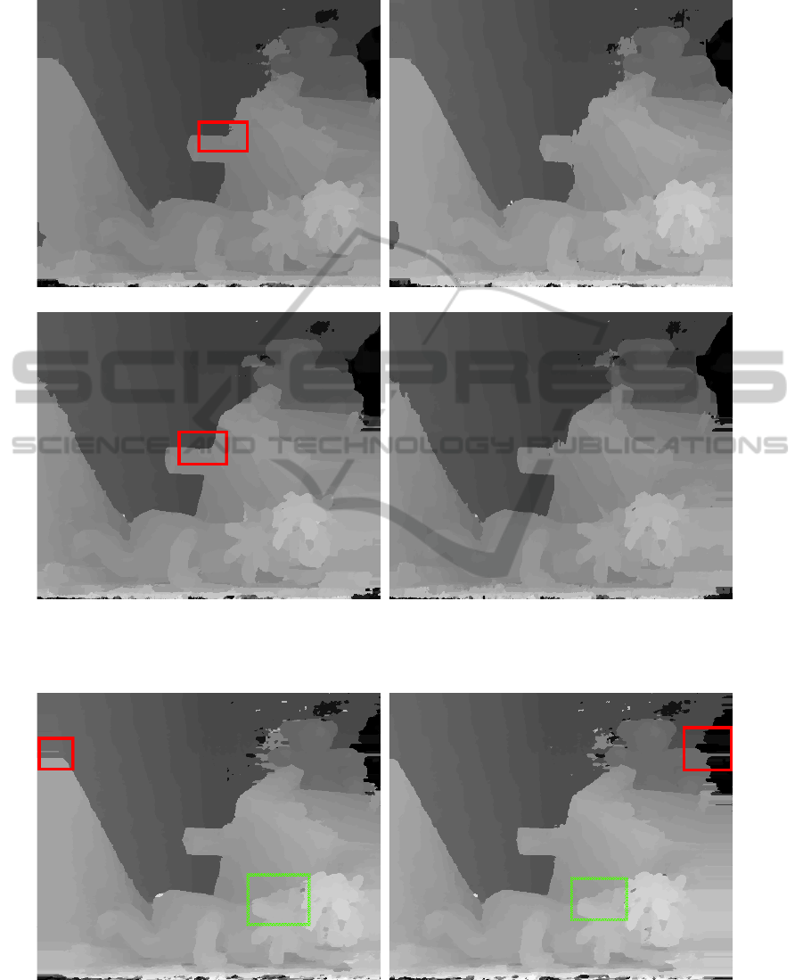
(a) Our method, left image (b) The method of (Zhang et al., 2009a), left image
(c) Our method, right image (d) The method of (Zhang et al., 2009a), right image
Figure 5: Comparison of our method (a), (c) and the similar method of (Zhang et al., 2009a)(b), (d), for both the left and right
images. The results clearly show that the edges in the image are more correct and contain less artifacts. This is especially true
for horizontal edges, as highlighted by the red squares.
(a) Without bitwise fast voting, left image (b) Without bitwise fast voting, right image
Figure 6: Results without bitwise voting. The results with bitwise voting are shown in Figure 5, (a) and (c). The red, full
squares show the result at the borders of the disparity maps. Not enough information is available in both images to estimate
the disparity correctly. Therefore, filling these values naively will result in erroneous lines. By using bitwise voting, these
artifacts are eliminated. The green, dashed squares show the handling of invalid disparity values around edges in the images
(i.e. occlusion). When no bitwise voting is applied, edges are fattened and the disparity values leak over the edges, resulting
in artifacts. This is avoided by incorporating color information.
Real-timeLocalStereoMatchingUsingEdgeSensitiveAdaptive Windows
123
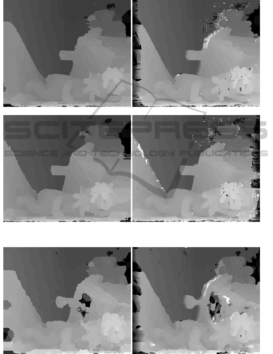
(a) With disparity refinement, left image (b) Without disparity refinement, left image
(c) With disparity refinement, right image (d) Without disparity refinement, right image
Figure 7: Comparison of the results with and without disparity refinement. Many artifacts are eliminated, including errors at
the borders of the disparity maps, speckle noise, mismatches that only occur in one disparity map, etc.
(a) With bitwise fast voting (b) Without bitwise fast voting
Figure 8: Comparison of the results with and without bitwise voting for stereo methods using fixed square aggregation win-
dows. The results are clearly better when applying bitwise voting. This demonstrates that this method is not only applicable
to the aggregation windows described above.
SIGMAP2014-InternationalConferenceonSignalProcessingandMultimediaApplications
124

when N(p) = 0 (Eq. 23). This occurs mostly near the
borders of the disparity maps, but can also manifest
itself anywhere in the image where the occlusions are
large enough.
We will therefore estimate a value for the remain-
ing invalid disparities, and store them in the corrected
disparity map D
I
(p). For each pixel with an invalid
disparity value, we search to the left and to the right
on its scanline for the closest valid disparity value.
The disparity map is not updated iteratively, so that
only the information of D
B
(p) is used for each pixel.
The result is shown in Fig. 4(i).
6.3 Median Filter
In the last refinement step, small disparity outliers are
filtered using a median filter, resulting in the absolute
final disparity map D
M
(p) shown in Fig. 4(j). A me-
dian filter has the property of removing speckle noise,
in this case caused by disparity mismatches, while re-
turning a sharp signal (unlike an averaging filter). In
our method, we calculate the median for each pixel
over a 3 × 3 window using a fast bubble sort (Astra-
chan, 2003) implementation in CUDA.
7 RESULTS
We demonstrate the effectiveness of our method using
the standard Middlebury dataset Teddy (Scharstein
and Szeliski, 2003). We compare our method with
the method of (Zhang et al., 2009a), which only uses
a horizontal primary axis, using our own implementa-
tion to provide a valid comparison. All comparisons
with ground truth data use the PSNR metric, where
higher is better.
Our method is better with an increase of 0.53 dB,
i.e. from 18.65 dB to 19.18 dB. Furthermore, the re-
sults are visually better, as observed in Fig. 5. The
figure clearly shows that the edges in the image con-
tain less artifacts, especially around horizontal edges.
As we will discuss next, the refinement steps of
section 6 contribute significantly to the final quality of
the disparity maps, which show significant improve-
ments both visually and quantitatively measured by
the PSNR metric.
Fig. 6 shows the result when the bitwise fast vot-
ing is disabled. Here, all invalid disparity values are
handled by using the closest value on the pixel’s scan-
line. We make two observations. First, the borders of
the disparity maps show a clear decrease in quality.
This is caused by the fact that many invalid disparity
values can be found here due to the missing informa-
tion in one of the images. Because using the closest
valid disparity value does not take the color values
into account, artifacts are created. Second, edge fat-
tening, meaning that the disparity values leak over the
edges, can be seen everywhere in the image. Again,
this is because no color information is used to esti-
mate the invalid disparity values. The use of bitwise
voting gives an increase of 0.75 dB, from 18.43 dB to
19.18 dB.
Finally, Fig. 7 shows the result when no refine-
ment is applied at all. Many improvements can be
noticed visually, including the elimination of speckle
noise, errors at the borders of the disparity map, etc.
Compared to the ground truth, we demonstrate an im-
provement of 3.52 dB, from 15.66 dB to 19.18 dB.
As a matter of fact, bitwise voting can be applied
to any local stereo algorithm. To demonstrate this,
we applied bitwise voting to a disparity map that was
computed using fixed square aggregation windows.
This is shown in Fig. 8. As shown, the results im-
prove, but all artifacts from a naive stereo matching
algorithm cannot be eliminated.
Our method runs at 13 FPS for 450 × 375 reso-
lution images on an NVIDIA GTX TITAN, therefore
providing a real-time solution.
8 CONCLUSION
We have shown that combining horizontal and ver-
tical edge aggregation windows in stereo matching
yields high quality levels in the disparity map esti-
mation. A 0.5 dB gain over state-of-the-art methods
and smooth disparity images with sharp edge preser-
vation around objects is achieved. Nonetheless, the
complexity of the final solution is comparable to ex-
isting methods, allowing efficient GPU implementa-
tion. Furthermore, we demonstrate that the disparity
refinement has a large effect on the final quality.
REFERENCES
Astrachan, O. (2003). Bubble sort: an archaeological algo-
rithmic analysis. ACM SIGCSE Bulletin, 35(1):1–5.
Davis, J., Ramamoorthi, R., and Rusinkiewicz, S. (2003).
Spacetime stereo: A unifying framework for depth
from triangulation. In Computer Vision and Pattern
Recognition, 2003. Proceedings. 2003 IEEE Com-
puter Society Conference on, volume 2, pages II–359.
IEEE.
Lu, J., Rogmans, S., Lafruit, G., and Catthoor, F. (2007a).
High-speed dense stereo via directional center-biased
support windows on programmable graphics hard-
ware. In Proceedings of 3DTV-CON: The True Vision
Capture, Transmission and Display of 3D Video, Kos,
Greece.
Real-timeLocalStereoMatchingUsingEdgeSensitiveAdaptive Windows
125

Lu, J., Rogmans, S., Lafruit, G., and Catthoor, F. (2007b).
Real-time stereo using a truncated separable lapla-
cian kernel approximation on programmable graphics
hardware. In Proceedings of International Conference
on Multimedia and Expo, pages 1946–1949, Beijing,
China.
Papadakis, N. and Caselles, V. (2010). Multi-label depth
estimation for graph cuts stereo problems. Journal of
Mathematical Imaging and Vision, 38(1):70–82.
Richardt, C., Orr, D., Davies, I., Criminisi, A., and Dodg-
son, N. A. (2010). Real-time spatiotemporal stereo
matching using the dual-cross-bilateral grid. In Com-
puter Vision–ECCV 2010, pages 510–523. Springer.
Scharstein, D. and Szeliski, R. (2002). A taxonomy and
evaluation of dense two-frame stereo correspondence
algorithms. International journal of computer vision,
47(1):7–42.
Scharstein, D. and Szeliski, R. (2003). High-accuracy
stereo depth maps using structured light. In Proceed-
ings of the IEEE Conference on Computer Vision and
Pattern Recognition (CVPR 2003), volume 1, pages
195–202. IEEE.
Wang, L., Liao, M., Gong, M., Yang, R., and Nister, D.
(2006). High-quality real-time stereo using adap-
tive cost aggregation and dynamic programming. In
3D Data Processing, Visualization, and Transmission,
Third International Symposium on, pages 798–805.
IEEE.
Yang, Q., Wang, L., Yang, R., Wang, S., Liao, M., and Nis-
ter, D. (2006). Real-time global stereo matching using
hierarchical belief propagation. In BMVC, volume 6,
pages 989–998.
Zhang, K., Lu, J., and Lafruit, G. (2009a). Cross-based
local stereo matching using orthogonal integral im-
ages. Circuits and Systems for Video Technology,
IEEE Transactions on, 19(7):1073–1079.
Zhang, K., Lu, J., Lafruit, G., Lauwereins, R., and
Van Gool, L. (2009b). Real-time accurate stereo with
bitwise fast voting on cuda. In Computer Vision Work-
shops (ICCV Workshops), 2009 IEEE 12th Interna-
tional Conference on, pages 794–800. IEEE.
Zitnick, C. L. and Kang, S. B. (2007). Stereo for image-
based rendering using image over-segmentation. In-
ternational Journal of Computer Vision, 75(1):49–65.
SIGMAP2014-InternationalConferenceonSignalProcessingandMultimediaApplications
126
