
A Modified Preventive Maintenance Model with Degradation Rate
Reduction in a Finite Time Span
Chun-Yuan Cheng, Jr-Tzung Chen, Te-Hsiu Sun and Mei-Ling Liu
Department of Industrial Engineering and Management, Chaoyang University of Technology, Taichung, Taiwan, R.O.C.
Keywords: Preventive Maintenance, Finite Time Span, Degradation Rate Reduction.
Abstract: Preventive maintenance (PM) can slow the deterioration process of a repairable system and restore the
system to a younger state. The proposed PM model of this paper focuses on the restoration effect of
degradation rate reduction which can only relieve stress temporarily and slow the rate of system degradation
while the hazard rate is still monotonically increased. This PM model considers a deteriorating but
repairable system (or equipment) with a finite life time period. This PM model is modified based on an
original degradation-rate-reduction PM model over a finite time span of which the searching range for the
optimal solution of the time interval between each PM is limited. It is demonstrated that the proposed
degradation-rate-reduction PM model over a finite time period can have a better optimal solution than the
original PM model. The algorithm of finding the optimal solution for the modified PM model is developed.
Examples are provided and are compared with the corresponding original PM model.
1 INTRODUCTION
For a deteriorating and repairable system, the
preventive maintenance (PM) can slow down the
aging process and restore the system to a younger
state (Pham and Wang 1996). Many PM models
shown in the literature assume the PM can restore
the system to a younger age or a smaller hazard rate,
such as Nakagawa (1986) and Chan and Shaw
(1993). However, the PM tasks, such as cleaning,
adjustment, alignment, and lubrication work, may
not always reduce system’s age or hazard rate.
Instead, this type of PM tasks may only reduce the
degradation rate of the system to a certain level. It
can be seen from the literature of the reliability-
centered maintenance (RCM) and the total
productive maintenance (TPM) (Bertling, Allan and
Eriksson 2005, Zhou, Xi, and Lee 2007, McKone,
Schroeder and Cua 2001, and Talib, Bon and Karim
2011) that this type of PM tasks is important for
keeping a system or equipment in the state of high
reliability. Canfield (1986) proposed an infinite-
time-span model for the above PM tasks which
assumes that the PM can only relieve stress
temporarily and slow the rate of system degradation
while the hazard rate is still monotonically increased.
Based on Canfield’s model, Park, Jung and Yum
(2000) and Cheng and Chen (2008) developed the
optimal periodic PM policy for the deteriorating
systems over an infinite time span.
In real world, a system’s useful life is normally
finite. When an aged system is replaced by a new
one, the new system seldom has exactly the same
conditions (such as characteristics, investment cost,
and maintenance expenses) as those of the system of
the previous replacement cycle. However, not many
PM models consider the conditon of finite time span.
Only some examples are found, such as Pongpech
and Murthy (2006), Yeh and Chen (2006) and
Ponchet, Fouladirad and Grall (2011). Hence, it is
worthwhile to study the PM problem with a finite
time span.
Furthermore, it is found from the PM models
developed by Pongpech and Murthy (2006) and
Cheng and Liu (2010) that a shorter time interval
between each PM can result in a better expected
total maintenance cost. However, these PM models
do limit the possibility of finding a smaller total
maintenance cost since the searching range of the
time interval between each PM is limited.
In this paper, a new degradation-rate-reduction
PM model over a finite time span is proposed by
releasing the restriction of the searching range for
the time interval between each PM. The algorithm of
finding the optimal solution for the proposed new
PM model is provided. Examples of Weibull failure
746
Cheng C., Chen J., Sun T. and Liu M..
A Modified Preventive Maintenance Model with Degradation Rate Reduction in a Finite Time Span.
DOI: 10.5220/0005068607460750
In Proceedings of the 11th International Conference on Informatics in Control, Automation and Robotics (ICINCO-2014), pages 746-750
ISBN: 978-989-758-040-6
Copyright
c
2014 SCITEPRESS (Science and Technology Publications, Lda.)

case are constructed for this new PM model to
examine the assumption and to analyze the
sensitivity of the optimal solution.
2 MODEL DEVELOPMENT
2.1 Nomenclature
L
The useful life time (finite time span) for
the system or equipment
T
The time interval of each periodic PM
N
The number of PM performed in the finite
life time span (L)
The restoration ratio of the degradation
rate corresponding to age in each PM and
0
1 where
=0 represents minimal
repair and
=1 represents perfect
maintenance. where is the restored ratio
δ(
)
The level of degradation rate reduction
after each PM, which is measured by the
corresponding age reduction and is
function of the restoration ratio
.
The time interval between the N
th
PM and
L, i.e., π = L NT
λ
(t)
The original hazard rate function (before
performing the 1
st
PM)
λ
i
(t)
The hazard rate function at time t where t
is in the i
th
PM cycle and λ
0
(t)=λ(t)
i
(t)
The expected number of failure at time t
of the i
th
PM cycle and Λ
0
(t)=Λ(t)
(, )
pm
Ci
Cost of the i
th
PM which is function of i
and δ(
)
C
m
r
The minimal repair cost of each failure
(,,)TC N T
The expected total maintenance cost
function over the finite life time interval L
2.2 The Assumptions
The following are the assumptions for the proposed
PM model.
The system is deteriorating over time with
increasing failure rate (IFR) in which Weibull
failure distribution is assumed in this paper, i.e.
1
() ( )
t
t
(1)
where
is the scale parameter and
is the shape
parameter with
> 1.
The PM can reduce the system’s degradation
rate to a younger level.
The reduced degradation rate of each PM is
assumed to be constant and is measured by the
restored ratio (
) of the corresponding age of
the degradation rate.
The time interval of each PM (T) is limited in
the range of (0, L].
Minimal repair is performed when a failure
occurs between each PM where the system is
restored to its condition just prior to the failure.
The system is disposed at the specified finite
time L without replacing a new one.
The total maintenance cost (TC) is considered
as the objective function which includes the
minimal repair cost and the PM cost in this new
model.
The minimal repair cost (C
mr
) is assumed to be
constant.
The cost of the i
th
PM (C
pm
) is assumed to be
variable, which is affected by the age (expressed
by the number of PM already performed) and
the reduced level of degradation rate, and is
defined in the following equation.
(, ) ( )
pm
Ci abic
,
(2)
where coefficient a represents the constant part
of the PM cost, b and c represent the unit
incremental PM cost of aging and the restored
level of degradation rate, respectively.
The times to perform PM and minimal repair
are negligible.
2.3 The Idea of the Modified Model
It is found that the time interval between each PM
(T) of the failure-rate-reduction PM models
developed by Pongpech and Murthy (2006) and
Cheng and Liu (2010) is constrained in the range of
min max
[, )TT
where
min
/( 1)TLN
and
max
/TLN
for a specified number of PM (N) in the
finite time span (L). It is also known that the optimal
value of T be the smallest possible value (i.e.,
min
T
)
when given a specified N. This result is also seen in
the degradation-rate-reduction PM model (no
warranty case) proposed by Cheng et al. (2009).
Thus, the constraint do limit the possibility of
finding the optimal value of T being smaller than
min
T
.
In this paper, the degradation-rate-reduction PM
model of no warranty case proposed by Cheng et al.
(2009) is called the original PM model. Figure 1
illustrates the hazard rate function of the original PM
model where
is the time interval between L and
the time of the last PM (NT), i.e.,
= L
NT. It can
be seen that
< T when T is restricted in the range
AModifiedPreventiveMaintenanceModelwithDegradationRateReductioninaFiniteTimeSpan
747
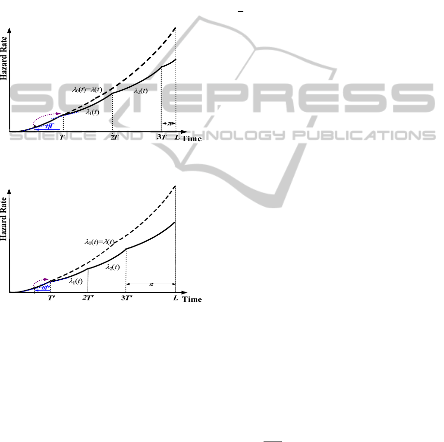
of
min max
[, )TT
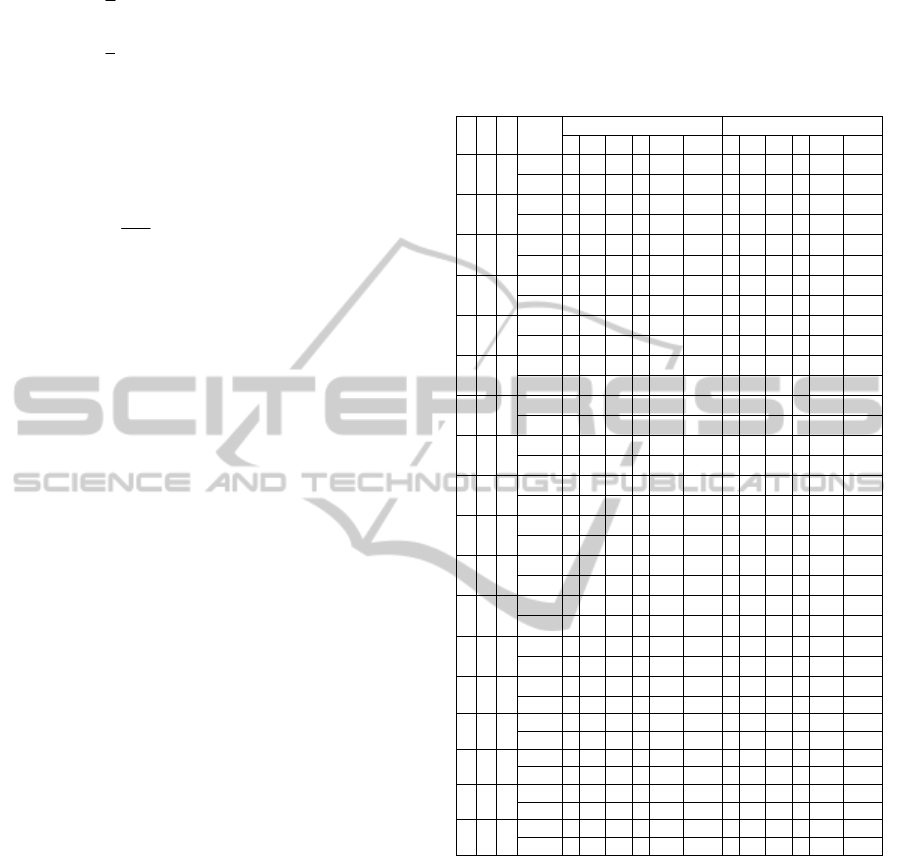
. Next, the modified degradation-rate-
reduction PM model over a finite time span is
proposed by releasing the restriction of T which is
illustrated in Figure 2. Under a specified finite time
span (L) and a given number of PM (N), it can be
observed that the interval of
shown in Figure 2 be
greater than the PM interval
'T
(i.e.,
>
'T
) and
'T
has smaller value than T of the original PM
model (as shown in Figure 1). Then, it is desired to
presume and verify the modified PM model can
provide a better optimal solution.
Figure 1: The illustration of the original degradation-rate-
reduction PM model.
Figure 2: The illustration of the modified degradation-rate-
reduction PM model.
2.4 The Modified PM Model
First, we have to obtain the total expected number of
failures over the entire finite time interval L, denoted
as (L), which is shown in Equation (4).
1
(1)
0
() .
N
iT L
iN
iT NT
i
Ltdttdt
(3)
Based on Canfied (1986), the hazard rate function of
the i
th
PM (
i
(t)) of the degradation-rate-reduction
PM model can be presented as
1
( ), 0 for 0,
(1)(1) (1)
()
( ), ( 1) ,
for 1, 2, , .
i
k
i
ttTi
Tk T k T
t
tiT iT t i T
iN
(4)
For a Weibull failure distribution, (L) can be
obtained as the following equation.
1
11
11
1
1
11
1
()
, =0
1
(1)
( 1)
( ) ( 1)
, 0
{
}
Ni
ik
N
i
N
k
L
L
N
T T kT k T kT kT
i T iT iT iT
LNT kT k T kTkT
LNT NTNT N
(5)
Next, the expected total maintenance cost (TC) of
the modified PM model is shown as follows.
1
(), =0
(,,)
() ,, , 0
mr
N
mr pm
i
CLN
TC N T
CL CiT N
(6)
By substituting Equations (4) and (5) into Equation
(6), we can obtain the expected TC cost in Equation
(7). Note that the equation of TC cost of the
modified PM model is same as the original PM
model. The difference of the two PM models is the
searching range of T.
0
0
1
11
1
1
1
(,,)
() , =0
()
( 1)
( 1)
( ) ( 1)
1
(), 0
2
{
}
L
mr
T
mr
Ni
ik
N
i
N
k
TC N T
CtdtN
Ctdt
TkTkT kTkT
i T iT iT iT
LNT kT k T kTkT
LNT NT NT
N
Na b cT N
(7)
For a Weibull failure distribution, the expected total
maintenance cost becomes
ICINCO2014-11thInternationalConferenceonInformaticsinControl,AutomationandRobotics
748
1
1
1
11
1
1
11
1
, =0
(1)
1
( 1)
(,,)
( ) ( 1)
1
(
2
{
}
mr
Ni
mr
ik
N
i
N
k
L
CN
kT k T
CTT
kT kT
i T iT iT iT
TC N T
LNT kT k T kTkT
LNT NTNT
N
Na b c
) , 0TN
(8)
3 THE OPTIMAL PM POLICY
The optimal solution for the modified PM model can
be obtained by minimizing the expected total
maintenance cost (TC). The decision variables are
the number of PM (N) over the finite time span (L),
the time interval of each PM (T
N
), and the
restoration ratio (
N
). It requires an algorithm with
numerical method to search for the optimal solution.
In this paper, we modify the algorithm provided by
Cheng and Liu (2010) with the Nelder-Mead
searching method which is a commonly used
nonlinear optimization technique for minimizing the
objective function in a multi-dimensional space. The
modified algorithm is presented as follows.
1.
Let N = 0, T
N
= L,
N
= 0.
2.
Calculate C
min
= TC(N, T
N
,
N
) using Equation
(7) or (8). (Note: C
min
equals to the expected total
maintenance cost of no PM.)
3.
Let N = 1.
4.
Calculate T
U
= L/N.
5.
Use Nelder-Mead method to search the values of
T
N
in the range of (0, T
U
] and
N
in the range of
[0, 1] such that TC(N, T
N
,
N
) shown in (7) or (8)
is minimized; let C
0
= minimal value of
TC (N, T
N
,
N
).
6.
If C
0
C
min
then obtain the optimal solution:
N
*
=N-1, T
*
=T
N*
,
*
=
N*
, TC(N
*
,T
*
,
*
), and stop;
else let N = N+1 and C
min
= C
0
; go to Step 4.
4 NUMERICAL EXAMPLES
Numerical examples are performed and the optimal
solutions of the modified PM model are compared
with those of the original PM model proposed by
Cheng et al. (2009). The system’s life is assumed to
follow Weibull distribution with scale parameter
=1 and shape parameter
= 2.5, and 3. Let L=5,
C
mr
=1 and the coefficients a, b, and c of C
pm
are
assigned with different values which satisfy C
pm
C
mr
as shown in Table 1.
Table 1: The comparison of the optimal solutions of the
modified and the original models.
abcModel
*
= 2.5
= 3
N
T
T
C
T
yp
e
**
N
T
T
C
T
yp
e
**
10.10.1
M 6 0.52 1.88 1 32.31 P 8 0.45 1.4
1 29.89 P
O 6 0.71 0.74 1 34.19 F 9 0.5 0.5
1 32.08 F
10.80.1
M 3 0.85 2.45 1 38.84 P 4 0.76 1.96
1 43.08 P
O 3 1.25 1.25 1 41.37 F 5 0.83 0.85
1 46.93 F
11.50.1
M 2 1.09 2.82 1 41.7 P 3 0.92 2.24
1 49.92 P
O 2 1.67 1.66 1 44.49 F 4 1 1
1 54.4 F
10.10.8
M 6 0.49 2.06 1 34.45 P 8 0.44 1.48
1 32.37 P
O 6 0.71 0.74 1 37.19 F 8 0.56 0.52
1 35.22 F
10.80.8
M 3 0.8 2.6 1 40.58 P 4 0.74 2.04
1 45.18 P
O 3 1.25 1.25 1 43.99 F 5 0.83 0.85
1 49.85 F
11.50.8
M 2 1.03 2.94 1 43.18 P 3 0.91 2.27
1 51.84 P
O 2 1.67 1.66 1 46.82 F 4 1 1
1 57.2 F
10.11.5
M 5 0.54 2.3 1 36.4 P 8 0.43 1.56
1 34.79 P
O 6 0.71 0.74 1 40.19 F 8 0.56 0.52
1 38.33 F
10.81.5
M
3 0.76 2.72 1 42.23
P
4 0.73 2.08
1 47.24
P
O
3 1.25 1.25 1 46.62
F
5 0.83 0.85
1 52.76
F
11.51.5
M
2 0.97 3.06 1 44.58
P
3 0.89 2.33
1 53.72
P
O
2 1.67 1.66 1 49.15
F
4 1 1
1 60
F
1.5 0.1 0.1
M
5 0.6 2 1 34.94
P
7 0.5 1.5
1 33.65
P
O
5 0.83 0.85 1 36.99
F
8 0.56 0.52
1 36.11
F
1.5 0.8 0.1
M
3 0.85 2.45 1 40.34
P
4 0.76 1.96
1 45.08
P
O
3 1.25 1.25 1 42.87
F
4 1 1
1 49.4
F
1.5 1.5 0.1
M
2 1.09 2.82 1 42.7
P
3 0.92 2.24 1 51.42
P
O
2 1.67 1.66 1 45.49
F
4 1 1
1 56.4
F
1.5 0.1 0.8
M
5 0.57 2.15 1 36.98
P
7 0.49 1.57
1 36.06
P
O
5 0.83 0.85 1 39.91
F
8 0.56 0.52
1 39.22
F
1.5 0.8 0.8
M
2 1.03 2.94 1 42.08
P
4 0.74 2.04
1 47.18
P
O
3 1.25 1.25 1 45.5
F
4 1 1 1 52.2
F
1.5 1.5 0.8
M
2 1.03 2.94 1 44.18
P
3 0.91 2.27 1 53.34
P
O
2 1.67 1.66 1 47.82
F
4 1 1 1 59.2
F
1.5 0.1 1.5
M
4 0.63 2.48 1 38.85
P
7 0.48 1.64 1 38.42
P
O
5 0.83 0.85 1 42.83
F
7 0.63 0.59 1 42.32
F
1.5 0.8 1.5
M
2 1.09 2.82 1 43.48
P
4 0.73 2.08 1 49.24
P
O
2 1.67 1.66 1 48.05
F
4 1 1 1 55
F
1.5 1.5 1.5
M
2 0.97 3.06 1 45.58
P
3 0.89 2.33 1 55.22
P
O
2 1.67 1.66 1 50.15
F
4 1 1 1 62
F
*
: In the 4
th
column, M represents the modified PM model while O
represents the original PM model.
**
: In the 10
th
and 16
th
columns, P represents the partially-periodic PM
interval while F represents the full
y
-
p
eriodic PM interval.
Table 1 shows the optimal solutions for the
examples. It can be found that the
*
= 1 for each
example. It can also be seen from these examples
that the new (modified) PM model has smaller PM
interval (T) and better optimal total maintenance cost
(TC) than the original PM model where the original
PM model has the fact: T
*
=
min
T = L/(N
*
+1). When
further examining the optimal policies of the
examples, it can be noticed that the modified PM
model has partially-periodic PM interval while the
original PM model has fully-periodic PM interval. It
can also be seen that a PM model with a shorter PM
AModifiedPreventiveMaintenanceModelwithDegradationRateReductioninaFiniteTimeSpan
749

interval does provide a better optimal solution. This
makes the presumption of this research acceptable.
We also analyze the sensitivity of each parameter
to the optimal solution for the modified PM model
by using the ANOVA method as shown in Table 2.
It can be found that
and c are significantly
sensitive to the optimal total maintenance cost TC.
The results indicate that the optimal TC is
significantly affected by a system’s failure rate (or
aging process) and the unit incremental PM cost of
the restored level of degradation rate.
Table 2: The Sensitivity Analysis for the Optimal Solution
of the New PM Model.
Response: TC
α
=0.05
Source Sum of Square DF Mean Square F Value Prob>F
Model 18730.60 9 2081.18 122.56 < 0.0001
β 16656.19 2 8328.09 490.43 < 0.0001
a 70.26 1 70.26 4.14 0.0450
b 1873.76 3 624.59 36.78 < 0.0001
c 130.39 3 43.46 2.56 0.0603
R
esidual
1460.39 86 16.98
C
or Total
20190.99 95
5 CONCLUSIONS
For the PM problem in a finite time span, based on
the fact that a shorter time interval of PM can result
in a better expected total maintenance cost, a
modified degradation-rate-reduction PM model is
developed with no constraint on the PM interval (T).
The algorithm of finding the optimal solution for the
new PM model is also constructed in this paper. It is
shown from the examples that the modified PM
model can provide better optimal solution than the
original PM model. This indicates that the modified
PM model is more suitable for the deteriorating and
repairable systems. For the future work, the
theoretical proof of the existence of the optimal
solution for the modified PM model needs to be
explored.
ACKNOWLEDGEMENTS
This research has been supported by Ministry of
Science and Technology of Taiwan under the project
number MOST101-2221-E-324-011-MY2.
REFERENCES
Bertling, L, Allan, R & Eriksson, R 2005, ‘A reliability-
centered asset maintenance method for assessing the
impact of maintenance in power distribution systems’,
IEEE Transaction on Power Systems, vol. 20, no. 1.
pp. 75-82.
Chan, JK & Shaw, L 1993, ‘Modeling Repairable Systems
with Failure Rates that Depend on Age and
Maintenance’, IEEE Transactions on Reliability, vol.
42, pp. 566-571.
Canfield, R. 1986, ‘Cost Optimization of Periodic
Preventive Maintenance’, IEEE Transactions on
Reliability, vol. R-35, pp. 78-81.
Cheng, CY & Chen, M 2008, ‘The periodic maintenance
policy for a Weibull life-time system with degradation
rate reduction under reliability limit’, the Asia-Pacific
Journal of Operational Research, vol. 25, no.6. pp.
793-805.
Cheng, CY & Liu, HH 2010, ‘The Finite Time Period
Preventive Maintenance Policies with Failure Rate
Reduction under A Warranty Consideration’, Journal
of the Chinese Institute of Industrial Engineers, vol.
27, pp. 81-89.
Cheng, CY, Sun, TH, Chen, JT & Liu, ML 2009, ‘The
Degradation -Rate-Reduction Preventive Maintenance
Policies with Warranty in a Finite Time Span’, in
IEEE International Conference on Industrial
Engineering and Engineering Management
(IEEM2009), Hong Kong.
McKone, KE, Schroeder, RG & Cua, KO 2001, ‘The
impact of total productive maintenance practices on
manufacturing performance’, Journal of Operations
Management, vol. 19, no. 1, pp. 39-58.
Nakagawa, T 1986, ‘Periodic and Sequential Preventive
Maintenance Policies’, Journal of Applied Probability,
vol. 23, pp. 536-542.
Park, DH, Jung, GM & Yum, JK 2000, ‘Cost
Minimization for Periodic Maintenance Policy of a
System Subject to Slow Degradation’, Reliability
Engineering and System Safety, vol. 68, pp. 105-112.
Pham, H & Wang, H 1996, ‘Invited Review: Imperfect
Maintenance’, European Journal of Operational
Research, vol. 94, pp. 425-438.
Ponchet, A, Fouladirad, M & Grall, A 2011, ‘Maintenance
policy on a finite time span for a gradually
deteriorating system with imperfect improvements’,
Proceedings of the Institution of Mechanical
Engineers, Part O: Journal of Risk and Reliability, vol.
225, pp. 105-116.
Pongpech, J & Murthy, DNP 2006, ‘Optimal Periodic
Preventive Maintenance Policy for Leased Equipment’,
Reliability Engineering & System Safety, vol. 91, pp.
772-777 .
Talib, A, Bon, B & Karim, N 2011, ‘Total Productive
Maintenance application to reduce Defects of Product’,
Journal of Applied Sciences Research, vol. 7, no. 1, pp.
11-17.
Yeh, RH & Chen, CK 2006, ‘Periodical preventive-
maintenance contract for a leased facility with weibul
life-time’, Quality & Quantity, vol. 40, pp. 303-313.
Zhou, X, Xi, L & Lee, J 2007, ‘Reliability-centered
predictive maintenance scheduling for a continuously
monitored system subject to degradation’, Reliability
Engineering and System Safety, vol. 92, pp. 530-534.
ICINCO2014-11thInternationalConferenceonInformaticsinControl,AutomationandRobotics
750
