
Spectral Clustering Using Evolving Similarity Graphs
Christina Chrysouli and Anastasios Tefas
Department of Informatics, Aristotle University of Thessaloniki, University Campus 54124, Thessaloniki, Greece
Keywords:
Spectral Clustering, Similarity Graphs, Evolutionary Algorithms.
Abstract:
In this paper, we propose a novel spectral graph clustering method that uses evolutionary algorithms in order
to optimise the structure of a graph, by using a fitness function, applied in clustering problems. Nearest
neighbour graphs and variants of these graphs are used in order to form the initial population. These graphs
are transformed in such a way so as to play the role of chromosomes in the evolutionary algorithm. Multiple
techniques have been examined for the creation of the initial population, since it was observed that it plays an
important role in the algorithm’s performance. The advantage of our approach is that, although we emphasise
in clustering applications, the algorithm may be applied to several other problems that can be modeled as
graphs, including dimensionality reduction and classification. Experiments on traditional dance dataset and
on other various multidimensional datasets were conducted using both internal and external clustering criteria
as evaluation methods, which provided encouraging results.
1 INTRODUCTION
The aim of clustering is to discover the natural group-
ing of a set of data, such that similar samples are
placed in the same group, while dissimilar samples
are placed into different ones. Clustering has been
used in a wide variety of applications, including
bioinformatics, data mining, image analysis, informa-
tion retrieval etc. A detailed survey on clustering ap-
plications can be found in (Jain et al., 1999) and a
more recent study in (Jain, 2008). In (Grira et al.,
2004) the authors attempt to briefly review a few core
concepts of unsupervised and semi-supervised clus-
tering.
Spectral graph clustering (Bach and Jordan, 2003)
refers to a class of graph techniques, that rely on
eigenanalysis of the Laplacian matrix of a similarity
graph, aiming to divide graph nodes in disjoint groups
(or clusters). In spectral clustering, as in all cluster-
ing techniques, nodes that originate from the same
cluster should have high similarity values, whereas
nodes from different clusters should have low simi-
larity values. Spectral analysis can be applied to a va-
riety of practical problems (i.e. computer vision and
speech analysis) and, as a result, spectral clustering
algorithms have received increasing interest. Some
clustering applicationsof spectral graph clustering are
reviewed in (Schaeffer, 2007).
So far, some evolutionary-based approaches to the
problem of clustering have been proposed through-
out the years. In (Maulik and Bandyopadhyay, 2000)
the authors proposed a genetic algorithm in order to
search for the cluster centers by minimising a cluster-
ing metric, while in (Murthy and Chowdhury, 1996)
authors aim to find the optimal partition of the data,
using a genetic algorithm, without searching all possi-
ble partitions. A more detailed survey of evolutionary
algorithms for clustering is presented in (Hruschka
et al., 2009).
In our approach, spectral graph clustering is ap-
plied on evolving similarity graphs, which have been
transformed properly in order to play the role of
the chromosomes in the employed genetic algorithm
(Holland, 1992). The initial population, for the ge-
netic algorithm, is constructed with the aid of k-
nearest neighbour graphs which, then, are trans-
formed to one-dimensional binary strings and un-
dergo genetic operators.
The remainder of this paper is organised as
follows. In section 2, the problem that we attempt
to solve is stated and some general aspects that
concern the algorithm are discussed, including
similarity graph construction, and spectral clustering
issues. Section 3, presents the proposed evolutionary
algorithm in detail. In Section 4, experimental results
of the algorithm are described. Finally, in Section 5,
conclusions are drawn and future work is discussed.
21
Chrysouli C. and Tefas A..
Spectral Clustering Using Evolving Similarity Graphs.
DOI: 10.5220/0005069200210029
In Proceedings of the International Conference on Evolutionary Computation Theory and Applications (ECTA-2014), pages 21-29
ISBN: 978-989-758-052-9
Copyright
c
2014 SCITEPRESS (Science and Technology Publications, Lda.)

2 PROBLEM STATEMENT
Clustering is the process of partitioning a usually
large dataset into groups, according to a similarity (or
dissimilarity) measure. The aim is that samples that
belong to the same cluster have a small distance from
each another, whereas samples that belong to differ-
ent clusters are at a large distance from each another.
Clustering is usually not a trivial task, as the only in-
formation we have about the data, is the data itself. In
order to obtain some information about the structure
of the data, we usually construct similarity matrices.
2.1 Similarity Functions and Similarity
Graphs
Similarities of data samples can be represented as a
similarity graph G = (V,E), whereV, E represent ver-
tices (or nodes) and edges of the graph, respectively.
If we assume that each vertexv
i
represents a data sam-
ple, then two nodes v
i
, v
j
are connected if the sim-
ilarity s
i, j
between them is positive or larger than a
threshold, and the edge is weighted by s
i, j
. The prob-
lem of clustering may now be reformulated as finding
a partition of the graph such that the weights within
a cluster have high values, whereas weights between
different clusters have low values.
Before constructing a similarity graph, we need
to define a similarity function on the data. The most
common similarity function S is the Gaussian simi-
larity function (heat kernel). Heat kernel between two
graph nodes is defined as:
S = h
i,j
= exp
−
v
i
− v
j
2
σ
2
!
, (1)
where σ is a parameter that defines the width of the
neighbourhood.
Generally, the most common choice of similarity
graphs are k-nearest neighbour graphs (to be called k-
nn graphs) because of their simplicity as well as their
sparsity. The aim of a k-nn graph A is to connect node
v
i
with node v
j
if v
j
is among the k nearest neigh-
bours of v
i
, which results in a directed graph. In the
proposed method, an undirected graph was used, ob-
tained by simply ignoring the directions of the edges.
However, it is well known that spectral clustering
is very sensitive to the choice of the similarity graph
that is used for constructing the Laplacian (Luxburg,
2007). Indeed, selecting a fixed k parameter for the
k-nn graph is very difficult and different values lead
to dramatically different clusterings. Optimising the
clustering over the graph structure is not a trivial task,
since the clustering criteria are not differentiable with
respect to the graph structure. Thus, we propose in
this paper to use evolutionary algorithms in order to
optimise specific clustering criteria, that are consid-
ered as fitness functions, with respect to the under-
lying graph, which is transformed to a chromosome
solution.
2.2 Spectral Graph Clustering
Spectral graph clustering (Bach and Jordan, 2003),
refers to a class of graph techniques, which rely on the
eigenanalysis of a matrix, in order to partition graph
nodes in disjoint clusters and is commonly used in
many clustering applications (Schaeffer, 2007).
Let D be a diagonal N × N matrix having the sum
d
ii
=
∑
j
W
i, j
on its main diagonal. Then, the gener-
alised eigenvalue problem is defined as:
(D− W)v = λDv, (2)
where W is the adjacency matrix, and v, λ are the
eigenvectors and eigenvalues respectively.
Although many variations of graph Laplacians ex-
ist (Luxburg,2007), we focus on the normalised graph
Laplacian L (Ng et al., 2002) defined as:
L = I− D
−1/2
WD
−1/2
(3)
where W is the adjacency matrix, with w
i, j
= w
j,i
≥ 0,
D is the degree matrix and I is the identity matrix. The
smallest eigenvalue of L is 0, which corresponds to
the eigenvector D
−1/2
1. The L matrix is always pos-
itive semi-definite and has n non-negativereal-valued
eigenvalues λ
1
≤ ... ≤ λ
n
. The computational cost of
spectral clustering algorithms is quite low when ma-
trices are sparse. Luckily, we make use of k-nn graphs
which are in fact sparse.
In the proposedmethod, we performeigenanalysis
on L matrix, where W is defined as:
W = S⊙ A, (4)
S represents the full similarity matrix obtained using
(1) and A represents an undirected k-nn matrix, which
is a sparse matrix. The ⊙ operator performs element-
wise multiplication. This process results in a sparse
matrix W, only containing elements in places where
A matrix contains elements. An example of the ⊙
operator is illustrated in Figure 1. Eigenvalues are al-
ways ordered increasingly, respecting multiplicities,
and the first k eigenvectors correspond to the k small-
est eigenvalues. Once the eigenanalysis has been per-
formed and the new representation of the data has
been obtained, the k-means algorithm is used in or-
der to attach a cluster to every data sample.
ECTA2014-InternationalConferenceonEvolutionaryComputationTheoryandApplications
22

S
1 0.1 0.4 0.6 0.8 0.7
0.1 1 0.5 0.8 0.1 0.4
0.4 0.5 1 0.6 0.9 0.5
0.6 0.8 0.6 1 0.6 0.9
0.8 0.1 0.9 0.6 1 0.2
0.7 0.4 0.5 0.9 0.2 1
⊙
A
1 0 0 0 1 0
0 1 0 1 0 0
0 0 1 1 1 0
0 1 1 1 0 1
1 0 1 0 1 0
0 0 0 1 0 1
=
W
1 0 0 0 0.8 0
0 1 0 0.8 0 0
0 0 1 0.6 0.9 0
0 0.8 0.6 1 0 0.9
0.8 0 0.9 0 1 0
0 0 0 0.9 0 1
Figure 1: The S matrix represents the full similarity matrix constructed using (1). The A matrix represents a k-nn graph,
which has undergone genetic operators. The ⊙ operator performs element-wise multiplication, resulting in a sparse matrix
W, which only contains elements in places where A matrix contains elements.
3 THE PROPOSED ALGORITHM
In order to partition a dataset into clusters, spectral
graph clustering has been applied on evolving k-nn
similarity graphs. In more detail, we evolve a num-
ber of k-nn similarity graphs with the aid of a ge-
netic algorithm, in order to optimise the structure of
the graph, by optimising a clustering criterion. In
this paper, clustering criteria were employed as fit-
ness functions. Moreover, k-nn similarity graphs are
transformed properly into chromosome solutions, in
order to be used in the genetic algorithm.
Let J be a clustering criterion that depends on the
similarity graph W. However, the optimisation prob-
lem is not convex and moreover the fitness function
is not differentiable with respect to W. Since S is
considered constant after selecting a specific similar-
ity function and through the definition of W in (4), the
optimisation problem is defined as:
optimise
A
J(A), (5)
where A
i, j
∈ 0,1 is a k-nn graph.
3.1 Construction of Initial Population
In our algorithm, we do not make use of the full simi-
larity matrix S, in order to create the initial population,
mainly for time and space efficiency reasons. Instead,
we use the sparse matrices that originate from k-nn
graphs, resulting in an initial population that consists
of matrices with binary elements. The employment of
the k-nn graphs, for the construction of the initial pop-
ulation, was based on the observation that their struc-
ture was already good (also they are sparse graphs),
thus, we could find a new structure of the graphs so
as to obtain better clustering results. Also, efforts to
use only random sparse matrices, as initial population,
have been made in order to gain completely different
structures of the graphs, which led to worse results,
thus, not presented here.
In this method, a Gaussian function has been em-
ployed as a similarity measure, in order to obtain the
similarity matrix S, which is calculated pairwise for
all the data in a database of our choice, using (1). Our
experiments showed that the value of σ has a decisive
role to the performance of the algorithm, thus, sev-
eral, arbitrary rules exist, concerning the choice of σ;
in the proposed method, we have used multiples of
the data diameter.
First, we calculate k-nearest neighbour matrices
A, with k = 3, ..., 8, which constitute the backbone of
the initial population. Next step is to enrich the pop-
ulation with nearly k-nearest neighbour matrices. In
order to achieve that, we alter the k-nearest neighbour
matrices that have already been calculated, by con-
verting a small proportion of 0’s, from A matrices, to
1’s and vice versa. This process guarantees that the
proportion of 1’s and 0’s will remain the same in the
new matrix. It is important not to alter the k-nn graphs
completely, so as to keep all the good properties. Fi-
nally, a small proportion of completely random ma-
trices are added, in order to increase the population
diversity, in which the number of 1’s are equal to the
number of 1’s that a 5-nn graph would have.
From the various experiments conducted, we have
concluded that the selection of the parameter k of
the nearest neighbour graphs is crucial to the clus-
tering results, as illustrated in Figure 2. Figure 2(a)
presents a dataset that consists of two classes with
each one having a different colour. Figures 2(b) and
2(c) represent the clustering results when a 3 and a 5-
nearest neighbour graph were used, respectively. We
should highlight the difference between the clustering
results, especially when the elements are close to both
classes.
Before proceeding to the algorithm, we must de-
fine the way that the k-nn matrices, and variants of
these matrices, in the initial population are trans-
formed into chromosomes, thus, we need to define
how a square matrix becomes a one-dimensional vec-
tor. As the k-nn graphs A are constructed in such a
way to be symmetrical, we may only keep the ele-
ments of the upper triangular matrix, with no loss of
information. Then, the remaining elements are ac-
cessed in rows, forming the one-dimensional vector
SpectralClusteringUsingEvolvingSimilarityGraphs
23

−12 −10 −8 −6 −4 −2 0 2 4 6 8
−8
−6
−4
−2
0
2
4
(a) Real classes
−10 −5 0 5
−8
−6
−4
−2
0
2
4
(b) 3-nearest neighbour graph
−10 −5 0 5
−8
−6
−4
−2
0
2
4
(c) 5-nearest neighbour graph
Figure 2: The effect of k-nearest neighbour graphs in clustering. In Figure 2(a) the two classes of the dataset are presented.
Figures 2(b) and 2(c) represent the clustering results when a 3 and a 5-nearest neighbour graph were used, respectively. Notice
the difference in clustering results especially when the data are close to both classes.
1 0 0 0 1 0
0 1 0 1 0 0
0 0 1 1 1 0
0 1 1 1 0 1
1 0 1 0 1 0
0 0 0 1 0 1
→
0 0 0 1 0
0 1 0 0
1 1 0
0 1
0
→
000100100110010
Figure 3: The way a k-nn graph A is transformed into a, one-dimensional vector, chromosome. We only keep the elements of
the upper diagonal, as the matrix is constructed to be symmetric, resulting in a matrix like the one in the middle. Then, this
matrix is accessed horizontally, in order to obtain the desirable result, the chromosome.
(Figure 3).
3.2 Optimisation of the Solutions
The novelty of the proposed algorithm is based on
the way that we select to optimise the solutions of
the problem, by optimising a clustering criterion J,
as previously defined in (5). Clustering criteria are di-
vided into two main categories, internal and external
criteria. The calculation of internal criteria implies
that we have no prior knowledge about the data and
we can only depend on quantities and features inher-
ent to the dataset, whereas calculation of external cri-
teria implies that we have some knowledge about the
dataset in advance (i.e. ground truth).
In the recent literature, many different cluster-
ing criteria (Vendramin et al., 2009) have been pro-
posed. Some of the most common internal criteria
are Calinski-Harabasz index (Cali´nski and Harabasz,
1974), Davies-Bouldin index (Davies and Bouldin,
1979) and Dunn’s index (Dunn, 1974), whereas some
external criteria are purity (Zhao and Karypis, 2001),
F-measure (Zu Eissen and Wißbrock, 2003), a mea-
sure based on hungarian algorithm (Munkres, 1957)
and normalised mutual information (He et al., 2005).
All the aforementioned criteria have been used both
for optimisation and evaluating the performance of
the algorithm.
As the value of such criteria cannot be optimised,
without the use of derivatives, we have employed evo-
lutionary techniques in order to solve this problem.
The optimisation is performed by altering the chro-
mosomes or, else, by altering the k-nn similarity ma-
trices A as in (2).
3.3 The Genetic Cycle
As we have already defined how the initial population
is formed and how the chromosome evaluation is per-
formed, we may now define the details of the genetic
algorithm.
Evolutionary algorithms solve problems based on
operators inspired from biology. The first step of the
genetic algorithm is to select the chromosomes which
will undergo the crossover operator. For this purpose,
a roulette wheel method has been employed (De Jong,
1975), where a probability is associated with each
chromosome, based on the value of the fitness func-
tion: the higher the value, the higher the probability
to be selected. The probability p
i
of the i-th chromo-
some to be selected, if f
i
is its fitness value is defined
as:
p
i
=
f
i
Σ
N
j=1
f
j
. (6)
Next, we combine the selected chromosomes,
based on the crossover rate which was set to 0.7, in
order to produce new ones. In the proposed algo-
rithm, a single crossover point is randomly selected
ECTA2014-InternationalConferenceonEvolutionaryComputationTheoryandApplications
24

for every set of chromosomes and the sub-sequences
that are formed are exchanged respectively. Then, we
randomly choose a small proportion of the chromo-
somes, based on the mutation rate which was set to
0.4, to undergo mutation, that is the random change
of some elements of a chromosome. In order to guar-
antee that the newly produced chromosomes will not
have been altered too much we perform mutation by
converting 1% of 0’s to 1’s and vice versa.
After the application of genetic operations to the
chromosomes, the new generation has been formed.
In order to perform spectral clustering (Section 2.2),
we need to reconstruct the k-nearest neighbour matrix
A, which will consist of binary digits, from the one-
dimensional vector chromosome. Then we apply the
similarity matrix S on A using the ⊙ operator, in or-
der to obtain the W as illustrated in Figure 1. Spectral
clustering (Ng et al., 2002) may now be performed on
L as in (3).
The next step is to calculate the fitness values of
all the newly produced chromosomes, and place them
along with the parent-chromosomes. Then, elitism is
performed: we sort all chromosomes, with the fittest
being on the top, and we keep only those chromo-
somes with the highest fitness value, so as the number
of the chromosomes kept to remain unchanged after
every generation.
The proposed algorithm terminates when a maxi-
mum of 50 generations has been reached, or when the
optimised criterion has not been altered for 5 consec-
utive generations.
3.4 Semi-supervised Learning
It is natural for many practical problems to con-
sider that we only possess a proportion of labels in a
dataset. Then, the problem of clustering can be trans-
formed into how this small proportion of labels can be
used in order to obtain a better clustering of the data.
Semi-supervised learning (Chapelle et al., 2006), in
machine learning, is a class of techniques which uses
both labeled and unlabeled data, usually a small set
of the former and a large set of the latter, in order to
obtain clusters. In this paper, semi-supervised learn-
ing has been used in clustering, in order to optimise
an external criterion.
In more detail, for some of the experiments, we
have assumed that we possess a small proportion of
labels l of the dataset, which are selected randomly
once and, then, the same labeled data are used in ev-
ery genetic cycle. Then, using only these l labels, we
have computed the fitness value f of the population,
by using one of the external criteria. The evaluation of
the algorithm is performed using only the rest of the
Table 1: Datasets used.
Dataset Duration Classes Size of # of
dataset features
Movie 1 02 : 06 : 21 21 1,222 152×152
Movie 2 01 : 44 : 31 41 1,435 150×150
Dataset Source Classes Size of # of
dataset features
Libras
Movement UCI 15 360 90
Iris UCI 3 150 4
folk dances 5 1012 1000
criteria (and not the one being optimised), which are
also being calculated during every experiment. The
overall value of a criterion is the value of an exter-
nal criterion calculated as if we possessed the labels
for the whole dataset. Thus, this technique uses both
labeled and unlabeled data in order to obtain clusters.
Essentially, only a small proportion of labels was used
in this method for obtaining the fitness values of chro-
mosomes, while the rest of the procedure remained
unchanged.
4 EXPERIMENTS
In order to evaluate the proposed algorithm, we
have conducted several experiments using 5 different
datasets and exploiting several input parameters. The
characteristics of the datasets used, are described in
Table 1.
Datasets “Movie 1” and “Movie 2” consist mainly
of facialimages originate from movies, detected using
a face detector. In the experiments the images were
scaled, in order to have the same size, considering all
the detected facial images of the movie clip and using
a mean bounding box, from all bounding boxes that
the face detector provided. A problem that might arise
is that of anisotropic scaling: the images returned by
the detector might have different height and width,
which is problematic when scaling towards a mean
bounding box, thus we calculate the bigger dimen-
sion of the bounding box and then we take the square
box that equals this dimension centered to the original
bounding box center. Datasets “Libras Movement”
and “Iris” originate from UCI (Newman and Merz,
1998) and consist of less data than the rest. Lastly, the
initial “Folk dances” dataset consists of videos of 5
different traditional dances: Lotzia, Capetan Loukas,
Ramna, Stankena and Zablitsena with 180, 220, 220
201 and 192 videos respectively, from which his-
tograms were extracted according to (Iosifidis et al.,
2013). An example of the dataset is illustrated in Fig-
ure 4.
The size of the populations remained unchanged
SpectralClusteringUsingEvolvingSimilarityGraphs
25

Table 2: Libras Movement. Optimising F−measure % criterion.
σ labels% C
CH DB Dunn Hungarian NMI F-measure % Purity F−measure
best 5nn best 5nn best 5nn best 5nn best 5nn best 5nn best 5nn best 5nn
0.89 10 14 161.47 131.35 0.67 0.76 0.10 0.07 48.06 45.93 0.64 0.63 0.68 0.64 0.50 0.48 0.51 0.49
1.33 20 15 167.21 110.02 0.61 0.79 0.08 0.04 45.93 45.83 0.63 0.62 0.59 0.57 0.50 0.48 0.50 0.48
2.66 20 14 141.89 101.17 0.69 0.70 0.05 0.08 47.41 42.96 0.62 0.61 0.58 0.55 0.50 0.46 0.51 0.48
5.32 10 14 127.39 110.85 0.70 0.75 0.12 0.07 45.28 44.72 0.63 0.61 0.69 0.66 0.48 0.47 0.51 0.49
Table 3: Iris. Optimising F-measure % criterion, σ=3.83.
σ labels% C
CH DB Dunn Hungarian NMI F-measure % Purity F−measure
best 5nn best 5nn best 5nn best 5nn best 5nn best 5nn best 5nn best 5nn
3.83 5 3 140.68 134.05 0.67 0.74 0.23 0.13 74.67 70.67 0.59 0.59 0.83 0.78 0.76 0.74 0.77 0.75
3.83 10 3 161.40 82.17 0.49 0.89 0.16 0.04 65.56 58.22 0.48 0.33 0.80 0.71 0.68 0.60 0.69 0.62
3.83 All 3 359.03 162.73 0.60 0.53 0.28 0.07 85.11 69.78 0.69 0.49 - - 0.85 0.72 0.85 0.72
Table 4: Folk dances dataset. Optimising Calinski-Harabasz criterion.
σ labels% C
Calinski-Harabasz Davies-Bouldin NMI Purity
best 5nn best 5nn best 5nn best 5nn
0.45 5 77.803 40.665 2.116 3.317 0.32 0.255 0.468 0.434
0.9 5 71.026 38.309 2.745 3.252 0.281 0.271 0.441 0.434
1.8 5 74.923 43.649 2.292 3.013 0.312 0.291 0.469 0.463
Table 5: Movie 1. From top to bottom optimising Calinski-Harabasz, F-measure %, Purity % criteria.
σ C
Calinski-Harabasz Davies-Bouldin Hungarian Purity
best 5nn best 5nn best 5nn best 5nn
5000 21 161.239 121.659 1.165 1.162 20.922 20.758 0.468 0.475
15000 21 161.011 123.922 1.208 1.103 21.495 21.167 0.462 0.477
20000 21 149.195 121.413 1.169 1.072 21.113 20.404 0.459 0.475
σ labels % C
Hungarian F-measure % Purity F−measure total
best 5nn best 5nn best 5nn best 5nn
20000 10 22 21.17 19.42 0.31 0.29 0.48 0.46 0.24 0.22
10000 20 22 21.79 19.99 0.29 0.26 0.47 0.48 0.23 0.23
15000 20 22 20.51 20.51 0.28 0.26 0.47 0.48 0.24 0.23
20000 20 22 20.73 19.37 0.29 0.27 0.49 0.47 0.24 0.23
σ labels % C
Hungarian Purity % Purity F−measure
best 5nn best 5nn best 5nn best 5nn
5000 20 21 20.786 19.858 0.493 0.485 0.487 0.479 0.232 0.226
10000 20 20 21.877 21.304 0.504 0.493 0.483 0.473 0.245 0.240
15000 20 20 21.086 20.949 0.503 0.497 0.477 0.472 0.241 0.240
Figure 4: An example of Ramna dance, from the ”Folk
dances” dataset.
for all the experiments conducted and was set to 200
chromosomes. Every experiment was executed 3
times, so the results presented here are the average
of these runs. We should highlight here that, in ev-
ery experiment, only one clustering criterion c is be-
ing optimised. The values of the rest of the criteria
are also calculated during every experiment only for
evaluation reasons. In other words, the values of the
rest of the criteria are not their best values as if they
were being optimised themselves. Instead, their val-
ues depend on the clustering obtained by optimising
the criterion c. Moreover, the optimisation of a sin-
gle criterion does not necessarily mean that the rest of
the criteria will also be improved, especially when the
way in which the criteria are calculated differs a lot.
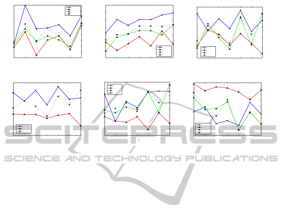
In Figure 5, results from “Movie 2” are illustrated,
with “Purity %” being the optimised criterion and as-
suming that we possess 20% of the total labels. Axes
ECTA2014-InternationalConferenceonEvolutionaryComputationTheoryandApplications
26
38 39 40 41 42 43 44
0.4
0.41
0.42
0.43
0.44
0.45
0.46
0.47
0.48
0.49
Purity 20% score − Maximum value is best
Number of clusters
Value of the criterion
best
5knn
8knn
bestInitial
(a) optimising Purity 20%
38 39 40 41 42 43 44
0.38
0.385
0.39
0.395
0.4
0.405
0.41
0.415
Purity score total − Maximum value is best
Number of clusters
Value of the criterion
best
5knn
8knn
bestInitial
(b) Purity
38 39 40 41 42 43 44
9.5
10
10.5
11
11.5
12
Hungarian score − Maximum value is best
Number of clusters
Value of the criterion
best
5knn
8knn
bestInitial
(c) Hungarian
38 39 40 41 42 43 44
0.1
0.105
0.11
0.115
0.12
0.125
F−measure score − Maximum value is best
Number of clusters
Value of the criterion
best
5knn
bestInitial
(d) F-measure
38 39 40 41 42 43 44
50
60
70
80
90
100
110
120
130
Calinski−Harabasz Criterion − Maximum value is best
Number of clusters
Value of the criterion
best
5knn
8knn
bestInitial
(e) Calinski-Harabasz
38 39 40 41 42 43 44
1.5
1.55
1.6
1.65
1.7
1.75
1.8
1.85
1.9
Davies−Bouldin Criterion − Minimum value is best
Number of clusters
Value of the criterion
best
5knn
8knn
bestInitial
(f) Davies-Bouldin
Figure 5: Results for dataset “Movie 2”. In every plot axis x, y represent the number of clusters and the value of each criterion
respectively. The optimisation was performed using the technique of semi-supervised learning and assuming that we possess
20% of the labels. The parameter of heart kernel was set to σ = 75.
x, y represent the number of clusters and the value of
each criterion, respectively. The “best” line, in the
Figure 5(a) represents the values of this criterion af-
ter its optimisation, whereas in the rest figures of the
criteria represents the value of the respective crite-
rion (i.e. Purity, Hungarian, etc.) according to the
best results of the optimised criterion (here, the “Pu-
rity%” criterion). The “5knn” and “8knn” lines repre-
sent the values of the criterion if clustering had been
performed using the 5 and 8-nearest neighbour graph,
respectively. The comparison with the results of the 5
and 8-nearest neighbour graphs is made as a baseline
for our method, since, especially the 5-nearest neigh-
bour graph, they are a common choice for data repre-
sentation. Finally, the “bestInitial” line represents the
results if the clustering would have been performed
on the best initial population among the k-nn graphs,
with k = 3,...,8. When optimising “Purity %” crite-
rion, the rest of the external criteria are also improv-
ing. Moreover, optimisation of “Purity %” seems to
improve the clustering when the number of clusters
was set equal to the number of classes, according to
internal criteria. Notice that, the way the internal cri-
terion “Davies-Bouldin” is defined, low values mean
better clustering has been performed.
In Tables presented here, we have attempted to
summarise some of the results of the datasets. The
results of the proposed method are represented under
the label “best”, while “5nn” represent the results of
the clustering if the 5-nn graph would have been em-
ployed to the data. Tables 2, 3 represent the results
of the algorithm, when “F−measure %” external cri-
terion was being optimised. For Tables 4, 5 and 6
the criteria being optimised are highlighted in every
sub-table (from top to bottom “Calinski-Harabasz”,
“F−measure %”, “Purity %”). The σ parameter is
the heat kernel parameter as in (1), C is the number of
clusters, and “labels %” is the percentage of the labels
we assumed to possess (only for external criteria).
5 CONCLUSION
We have presented a novel algorithm that makes use
of evolutionary algorithms in order to achieve good
clustering results, with the aid of nearest neighbour
graphs. It is important to remark that the algorithm
is general and can be used to manipulate a wide va-
riety of different problems, such as clustering and di-
mensionality reduction. The technique of using near-
est neighbour graphs as initial population appears to
yield satisfactory results, in terms of both internal and
external criteria.
In the future, we aim to improvethe proposed evo-
lutionary algorithm, by optimising even different cri-
teria, or even use multiple of them in order to decide
which chromosome is best. We shall also focus our
efforts on creating an even better initial population,
SpectralClusteringUsingEvolvingSimilarityGraphs
27

Table 6: Movie 2. From top to bottom optimising Calinski-Harabasz, F-measure %, Purity % criteria.
σ C
Calinski-Harabasz Davies-Bouldin Hungarian Purity
best 5nn best 5nn best 5nn best 5nn
25 40 81.917 70.737 1.240 1.204 15.889 15.447 0.400 0.398
50 41 76.269 69.302 1.144 1.257 16.353 15.819 0.410 0.408
75 41 78.449 66.245 1.226 1.200 16.121 15.981 0.401 0.402
150 40 82.090 66.393 1.183 1.248 16.167 15.772 0.403 0.391
σ labels % C
Hungarian F−measure % Purity F−measure total
best 5nn best 5nn best 5nn best 5nn
50 10 40 16.19 15.77 0.33 0.32 0.41 0.39 0.17 0.17
25 20 41 15.96 15.42 0.26 0.24 0.40 0.40 0.17 0.17
50 20 41 16.26 15.96 0.25 0.23 0.41 0.41 0.17 0.17
75 20 41 16.33 16.28 0.25 0.25 0.40 0.40 0.17 0.17
σ labels % C
Hungarian Purity % Purity F−measure
best 5nn best 5nn best 5nn best 5nn
50 20 41 32.733 32.706 0.404 0.404 0.380 0.378 0.458 0.461
75 20 41 10.229 10.120 0.451 0.430 0.401 0.394 0.109 0.108
150 20 41 17.267 16.667 0.515 0.497 0.455 0.440 0.181 0.178
for example by including more than only random vari-
ations of the nearest neighbour graphs.
ACKNOWLEDGEMENTS
This research has been co–financed by the European
Union (European Social Fund - ESF) and Greek na-
tional funds through the Operation Program “Educa-
tion and Lifelong Learning” of the National Strate-
gic Reference Framework (NSRF) - Research Fund-
ing Program: THALIS–UOA–ERASITECHNIS MIS
375435.
REFERENCES
Bach, F. and Jordan, M. (2003). Learning spectral cluster-
ing. Technical report, UC Berkeley.
Cali´nski, T. and Harabasz, J. (1974). A dendrite method for
cluster analysis. Communications in Statistics Simu-
lation and Computation, 3(1):1–27.
Chapelle, O., Sch¨olkopf, B., and Zien, A. (2006). Semi-
Supervised Learning. MIT Press.
Davies, D. L. and Bouldin, D. W. (1979). A cluster sepa-
ration measure. Pattern Analysis and Machine Intelli-
gence, IEEE Transactions on, (2):224–227.
De Jong, K. A. (1975). An analysis of the behavior of a
class of genetic adaptive systems. PhD thesis, Univer-
sity of Michigan, Ann Arbor. University Microfilms
No. 76-9381.
Dunn, J. C. (1974). Well-separated clusters and optimal
fuzzy partitions. Journal of cybernetics, 4(1):95–104.
Grira, N., Crucianu, M., and Boujemaa, N. (2004). Unsu-
pervised and semi-supervised clustering: a brief sur-
vey. A review of machine learning techniques for pro-
cessing multimedia content, Report of the MUSCLE
European Network of Excellence (FP6).
He, Z., Xu, X., and Deng, S. (2005). K-anmi: A mutual
information based clustering algorithm for categorical
data. CoRR.
Holland, J. H. (1992). Adaptation in Natural and Artificial
Systems: An Introductory Analysis with Applications
to Biology, Control and Artificial Intelligence. MIT
Press, Cambridge, MA, USA.
Hruschka, E. R., Campello, R. J. G. B., Freitas, A. A., and
De Carvalho, A. P. L. F. (2009). A survey of evolu-
tionary algorithms for clustering. Systems, Man, and
Cybernetics, Part C: Applications and Reviews, IEEE
Transactions on, 39(2):133–155.
Iosifidis, A., Tefas, A., and Pitas, I. (2013). Minimum class
variance extreme learning machine for human action
recognition. Circuits and Systems for Video Technol-
ogy, IEEE Transactions on, 23(11):1968–1979.
Jain, A. K. (2008). Data clustering: 50 years beyond k-
means. In ECML/PKDD (1), volume 5211, pages 3–4.
Springer.
Jain, A. K., Murty, M. N., and Flynn, P. J. (1999). Data
clustering: a review. ACM Computing Surveys,
31(3):264–323.
Luxburg, U. (2007). A tutorial on spectral clustering. Statis-
tics and Computing, 17(4):395–416.
Maulik, U. and Bandyopadhyay, S. (2000). Genetic
algorithm-based clustering technique. Pattern Recog-
nition, 33(9):1455–1465.
Munkres, J. (1957). Algorithms for the assignment and
transportation problems. Journal of the Society of In-
dustrial and Applied Mathematics, 5(1):32–38.
Murthy, C. A. and Chowdhury, N. (1996). In search of opti-
mal clusters using genetic algorithms. Pattern Recog-
nition Letters, 17(8):825–832.
ECTA2014-InternationalConferenceonEvolutionaryComputationTheoryandApplications
28

Newman, C. B. D. and Merz, C. (1998). UCI repository of
machine learning databases.
Ng, A. Y., Jordan, M. I., Weiss, Y., et al. (2002). On spectral
clustering: Analysis and an algorithm. Advances in
neural information processing systems, 2:849–856.
Schaeffer, S. E. (2007). Graph clustering. Computer Sci-
ence Review, 1:27–64.
Vendramin, L., Campello, R. J. G. B., and Hruschka, E. R.
(2009). On the comparison of relative clustering va-
lidity criteria. In SDM, pages 733–744. SIAM.
Zhao, Y. and Karypis, G. (2001). Criterion functions for
document clustering: Experiments and analysis.
Zu Eissen, B. S. S. M. and Wißbrock, F. (2003). On clus-
ter validity and the information need of users. ACTA
Press, pages 216–221.
SpectralClusteringUsingEvolvingSimilarityGraphs
29
