Modelling and Analysis of Retinal Ganglion Cells

Through System Identification

Dermot Kerr

, Martin McGinnity

and Sonya Coleman

School of Computing and Intelligent Systems, University of Ulster, Magee campus, Derry, Northern Ireland

School of Science & Technology, Nottingham Trent University, Nottingham, U.K.

Keywords: System Identification, Retinal Ganglion Cells, Linear-Nonlinear Model.

Abstract: Modelling biological systems is difficult due to insufficient knowledge about the internal components and

organisation, and the complexity of the interactions within the system. At cellular level existing

computational models of visual neurons can be derived by quantitatively fitting particular sets of

physiological data using an input-output analysis where a known input is given to the system and its output

is recorded. These models need to capture the full spatio-temporal description of neuron behaviour under

natural viewing conditions. At a computational level we aspire to take advantage of state-of-the-art

techniques to accurately model non-standard types of retinal ganglion cells. Using system identification

techniques to express the biological input-output coupling mathematically, and computational modelling

techniques to model highly complex neuronal structures, we will "identify" ganglion cell behaviour with

visual scenes, and represent the mapping between perception and response automatically.

1 INTRODUCTION

Modelling biological systems is difficult due to

insufficient knowledge about the internal

components and organisation, and the complexity of

the interactions within the system. System

identification has emerged as a viable alternative to

classical hypothesis testing for the understanding of

biological systems and was first used to understand

the responses of auditory neurons (De Boer, 1968).

Using white noise stimuli as input, the output

responses were recorded and inferences made on

mapping the stimulus to the response. White noise

stimulation is often selected to model biological

vision systems (Sakai, 1988, Chichilnisky, 2001) as

it is mathematically simple to analyse. However, it is

unlikely that white noise stimuli would test the full

function of a neuron’s behaviour (Talebi, 2012).

Thus, any model developed with this stimulus could

only be considered a subset of the biological model

under certain conditions.

In the work by Marmarelis (Marmarelis, 1972), the

Wiener theory of nonlinear system identification

was applied to study the underlying operation of the

three stage neuronal structures in the catfish retina.

Following from this work, the Volterra-Wiener

method has been used extensively to model

nonlinear biological systems (Victor, 1977, 1979,

Marmarelis, 2004, Korenberg, 1996). However,

computational effort increases geometrically with

the kernel order and in interpretation of higher order

kernels (Herikstad, 2011). Marmarelis and Zhao

(Marmarelis, 1997) presented a way of overcoming

these limitations by developing a perceptron type

network with polynomial activation functions.

Block-structured (Giri, 2010) or modular models

in the form of cascaded or parallel configurations

have been used to overcome the limitations of

Volterra-Wiener models. Cascade models may take

various forms such as linear-nonlinear (Ostojic,

2011), nonlinear-linear, linear-nonlinear-linear, etc.

In particular, linear-nonlinear models have been

used to describe the processing in the retina (Pillow,

2005).

The generalised modular model proposed by

Korenberg (Korenberg, 1991) employed parallel

linear-nonlinear cascades generating spike outputs

with a threshold-trigger function. To model specific

neuron responses such as burstiness, refractoriness

and gain control, Pillow (Pillow, 2008) amended the

linear-nonlinear models with feedback terms.

Correlated neuron activity was modelled through the

158

Kerr D., McGinnity M. and Coleman S..

Modelling and Analysis of Retinal Ganglion Cells Through System Identiﬁcation.

DOI: 10.5220/0005069701580164

In Proceedings of the International Conference on Neural Computation Theory and Applications (NCTA-2014), pages 158-164

ISBN: 978-989-758-054-3

 2014 SCITEPRESS (Science and Technology Publications, Lda.)

use of coupling filters (Pillow, 2008) to couple

multiple linear-nonlinear models of individual cells.

Parametric system identification modelling

techniques also exist. The NARMAX (nonlinear

auto-regressive moving average with exogenous

inputs) model (Billings, 1984) has been used to

model the nonlinear behaviour observed in the fly

photoreceptors (Friederich, 2009, Song, 2009). The

NARMAX modelling technique is suitable for

application in a number of areas and has also been

used to model robot behaviour (Kerr, 2010), iceberg

calving and detecting and tracking time-varying

causality for EEG data (Billings, 2013). Neural

network approaches have also been used to model

biological aspects of the vision system. For example

Lau (Lau, 2002) used a two layer neural network

with the backpropagation training algorithm to

model the nonlinear responses of neurons in the

visual cortex to visual stimuli. Similarly, Prenger

(Prenger, 2004) used a multilayer feed-forward

neural network to model the nonlinear stimulus-

response relationship in the primary visual cortex

using natural images.

In this paper we formalise and standardise the

model development process by using system

identification techniques (NARMAX modelling) to

express the biological input-output coupling

mathematically. We have used a NARMAX

approach to obtain the models we need because:

 The NARMAX model itself provides the

executable code straight away,

 The model is analysable, and gives us valuable

information regarding

 How the model achieves the task,

 Whether the model is stable or not,

 How the model will behave under certain

operating conditions, and

 How sensitive the model is to certain inputs,

i.e. how “important” certain input are.

In Section 2 we present the visual stimuli used in the

neuronal recordings to obtain the physiological data

and in Section 3 we present an overview of the

NARMAX modelling approach. Experiments and

results are presented in Section 4 with discussion in

Section 5.

2 NEURONAL DATA

Recordings were obtained from isolated mice retinas

under full field stimulation using a Gaussian white

noise sequence as illustrated in Figure 1.

Figure 1: Full-field Gaussian white noise sequence.

The isolated retina was placed on a multi-electrode

array, which recorded spike trains from many

ganglion cells simultaneously. Stimuli were

projected onto the isolated retina via a miniature

cathode ray tube monitor. Spikes were sorted off-

line by a cluster analysis of their shapes, and spike

times were measured relative to the beginning of

stimulus presentation. In the experiments presented

in this paper we analyse the response from an ON

retinal ganglion cell (RGC).

3 NARMAX MODELLING

The NARMAX model is a difference equation that

expresses the present value of the output as a

nonlinear combination of previous values of the

output, previous and/or present values of the input,

and previous and/or present values of the noise

signal. NARMAX is a parameter estimation

methodology for identifying both the important

model terms and the parameters of an unknown non-

linear dynamic system, such as a sensory neuron.

For single-input single-output systems this model

takes the form:

)(

)](,),1(

),(,),(

),(,),2(),1([)(

nekeke

nudkudku

nykykykyFky













(1)

where )(ky , )(ku , )(ke are the sampled output,

input and unobservable noise sequences

respectively,

nenuny ,,

are the regression orders of

)(ky , )(ku , )(ke and d is a time delay. []F is a

nonlinear function and is typically taken to be a

polynomial expansion of the arguments. Usually

only the input and output measurements are

ModellingandAnalysisofRetinalGanglionCellsThroughSystemIdentification

159

available and the investigator must process these

signals to estimate a model of the system.

The NARMAX methodology divides this

problem into the following steps:

 Structure detection;

 Parameter estimation;

 Model validation;

 Prediction;

 Analysis.

These steps form an estimation toolkit that allows

the user to build a concise mathematical description

of the system (Billings and Chen, 1998). The

procedure begins by determining the structure or the

important model terms using a special orthogonal

least squares procedure. This algorithm determines

which dynamic and nonlinear terms should be in the

model by computing the contribution that each

potential model term makes to the system output.

This allows the model to be built up term by term in

a manner that exposes the significance of each new

term that is added.

Structure detection is a fundamental part of

the NARMAX procedure because searching for the

structure ensures that the model is as simple as

possible and a model with good generalisation

properties is obtained. This approach mimics

analytical modelling methods where the important

model terms are introduced first. Subsequently the

model is refined by adding in less significant effects.

The only difference is that in the NARMAX method

the model terms can be identified from the data set.

These procedures are now well established

and have been used in many modelling domains.

Once the structure of the model has been determined

the unknown parameters in the model can be

estimated. If correct parameter estimates are to be

obtained the noise sequence, e(k) which is almost

always unobservable, must be estimated and

accommodated within the model. Model validation

methods are then applied to determine if the model

is adequate.

Once the model has been determined to be

adequate it can be used to predict the system output

for different inputs. The model may also be used to

study the characteristics of the system under

investigation (Nehmzow, 2006). It is this latter

aspect that is of particular interest in the work

presented here. In this paper we have examined the

suitability of NARMAX modelling to express the

biological stimulus-response coupling

mathematically and to validate the resulting

stimulus-response couplings.

4 MODEL IDENTIFICATION

PROCEDURE AND ANALYSIS

The proposed approach represents a decisive

departure from current methods of generating retina

models. We propose to "identify" (in the sense of

system identification) the neuron’s behaviour with

natural visual scenes, and to represent the mapping

between perception and response automatically,

using the NARMAX system identification

technique. We will illustrate how the various neural

networks within the layered retina structure can be

modelled using efficient polynomials that

incorporate the neuron's nonlinear behaviour and

dynamics. The compact polynomial representation

will demonstrate that the intricate retina neural

networks may be modelled in a compact compressed

form.

4.1 Data Pre-processing

The overall goal of the pre-processing stage is to

manipulate the data so that they form a regression

dataset, i.e. input-output corresponding to the

stimulus-response. In this case the dataset will be

single-input single-output.

The Gaussian white noise is a stochastic highly

interleaved stimuli spanning a wide range of visual

inputs, is relatively robust to fluctuations in

responsivity, avoids adaptation to strong or

prolonged stimuli and is well suited to simultaneous

measurements from multiple neurons. Examples of

stimuli are presented in Figure 1 where each image

in the sequence is presented sequentially to the

isolated retina. As the stimulus has uniform intensity

there is no need to extract the stimulus in the region

of the receptive field.

Recordings of the ganglion cell neural response

(spikes) to the full-field stimulation were supplied

for two different ganglion cells in the case of this

dataset. Each file contains the recorded times of

spikes in seconds. For example,

[1.76304, 1.76912, 1.78504,…,546.63776].

Using these recorded spike times we compute a

continuous temporal spike rate using the standard

method of binning and convolution with a window

function. Using this method we then have a

continuous valued input-output dataset. For

example, in Figure 2 we have illustrated the input

data (stimulus intensity), recorded spikes and

computed spike rate using an alpha window function

for 500 milliseconds of a recording. Figure 2(a)

illustrates the stimulus intensity, Figure 2(b)

illustrates the recorded spikes, and Figure 2(c)

NCTA2014-InternationalConferenceonNeuralComputationTheoryandApplications

160

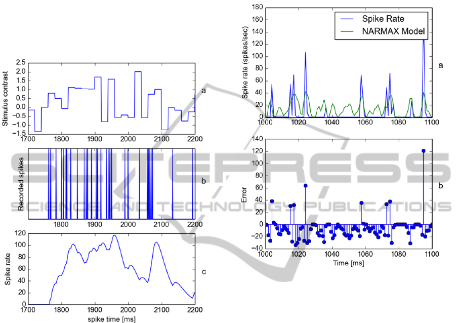
illustrates the spike computed using a half wave

rectified α function.

After this pre-processing stage we can use the

system identification method to obtain a polynomial

model that models the ganglion cells spike rate as a

function of the stimulus intensity where the spatially

uniform stimulus intensity is used as input (Figure

2(a)) and the computed spike rate (Figure 2(c)) is

used as output.

Figure 2: (a) Temporal stimulus intensity; (b) recorded

spikes; (c) computed spike rate for 500ms of a recording.

4.2 Identifying the RGC Linear Model

Using the NARMAX procedure outlined in Section

3 we construct a NARMAX model with an input

regression of nu = 10, corresponding to 200ms of

stimulus time and a polynomial of order 1. The

resulting model contained 11 terms and is presented

in equation (2).

nr(t)= +10.8820504569

+0.4133355718 * u1(n-1)

+5.7712836251 * u1(n-2)

+11.1532223508 * u1(n-3)

+5.4095799493 * u1(n-4)

-0.9100060568 * u1(n-5)

-2.2967796022 * u1(n-6)

-1.5449416639 * u1(n-7)

-0.8126715957 * u1(n-8)

-1.1259153820 * u1(n-9)

-1.4256504406 * u1(n-10)

(2)

Using a new test stimulus sequence we then evaluate

the performance of this NARMAX model and

compare it to the actual neuronal response to the test

stimulus. Results are presented in Figure 3.

Figure 3: Comparison of linear polynomial NARMAX

model and actual neuron response to novel test stimulus

sequence.

Figure 3 (a) illustrates the actual recorded spike rate

(blue) and the linear NARMAX model predicted

spike rate (green). Figure 3 (b) illustrates the model

error. We have also computed the RMSE as 20.92

and present a full comparison of RMSE results in

Table 1.

4.3 Identifying a RGC Quadratic

Model

Again using the same NARMAX procedure we

construct a quadratic NARMAX model with an

input regression of nu = 10, corresponding to 200ms

of stimulus time and a polynomial of order 2. The

resulting quadratic polynomial model contained 26

terms and is presented in equation (3).

Figure 4 (a) illustrates the actual recorded

spike rate (blue) and the quadratic NARMAX model

predicted spike rate (green). Figure 4 (b) illustrates

the model error. We have also computed the RMSE

as 18.31 and present a full comparison of RMSE

results in Table 1. Visual examination reveals both

ModellingandAnalysisofRetinalGanglionCellsThroughSystemIdentification

161

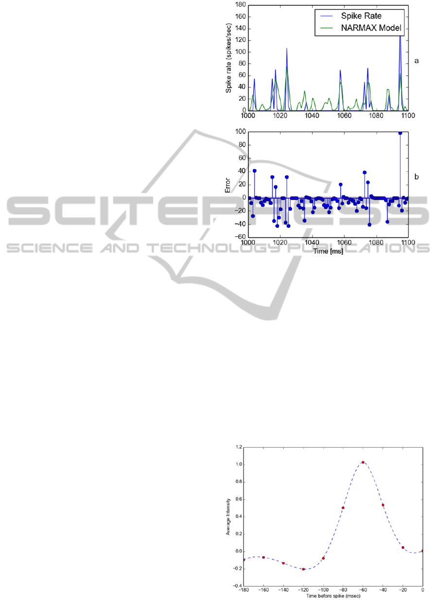
the linear and quadratic NARMAX models perform

similarly with similar errors although the quadratic

model has a reduced error compared to the linear

model.

nr(t)= +5.96244435

+5.70629880 * u1(n-2)

+11.10949549 * u1(n-3)

+5.38644092 * u1(n-4)

-0.89662644 * u1(n-5)

-2.17791043 * u1(n-6)

-1.41390802 * u1(n-7)

-0.75777998 * u1(n-8)

-1.08523454 * u1(n-9)

-1.33837116 * u1(n-10)

+1.65057833 * u1(n-2)^2

+4.28603998 * u1(n-3)^2

-1.01260994 * u1(n-5)^2

+4.84809445 * u1(n-2) * u1(n-3)

+1.55113103 * u1(n-2) * u1(n-4)

-0.63963641 * u1(n-2) * u1(n-5)

-0.71240927 * u1(n-2) * u1(n-6)

+3.30083736 * u1(n-3) * u1(n-4)

-1.14246640 * u1(n-3) * u1(n-5)

-1.76540112 * u1(n-3) * u1(n-6)

-0.95766543 * u1(n-3) * u1(n-7)

-0.66097265 * u1(n-3) * u1(n-9)

-1.10149068 * u1(n-3) * u1(n-10)

-2.13889232 * u1(n-4) * u1(n-5)

-1.68797033 * u1(n-4) * u1(n-6)

-1.03141419 * u1(n-5) * u1(n-6)

(3)

4.4 Comparison with Linear-nonlinear

Model

To provide further comparison for the NARMAX

models we evaluate against a standard benchmark by

computing the Linear-Nonlinear (LNL) model

(Ostojic, 2011). The first stage in computing the

Linear-Nonlinear model is to compute the spike

triggered average (STA) which is the average

stimulus preceding a spike.

To compute the STA, the stimulus in the time

window preceding each spike is extracted, and the

resulting (spike-triggered) stimuli are averaged.

Using the same dataset as the previous analysis we

compute the STA and the results are presented in

Figure 5. Here we can see that the RGC is an ON

cell due to the positive peak in the temporal response

of the filter. We can also see that the cell has a

temporal memory of approximately 150-100ms. The

plot illustrates the average values of stimulus

intensity that elicit a response from the cell.

Figure 4: Comparison of quadratic polynomial NARMAX

model and actual neuron response to novel test stimulus

sequence.

The second stage in the Linear-Nonlinear

model is used to re-construct the ganglion cells

nonlinearity. We using the standard approach

(Ostojic, 2011) of plotting the actual response

against the STA predicted response, binning the

values and fitting a curve using a cumulative density

function. Figure 6 illustrates the obtained non-

linearity. Next, we apply the STA and nonlinearity

to the same test stimulus and compute the response.

We compare this estimated response to the actual

neuronal response and plot the results as before.

Results are presented in Figure 7.

Figure 5: Computed spike triggered average for ON cell.

NCTA2014-InternationalConferenceonNeuralComputationTheoryandApplications

162

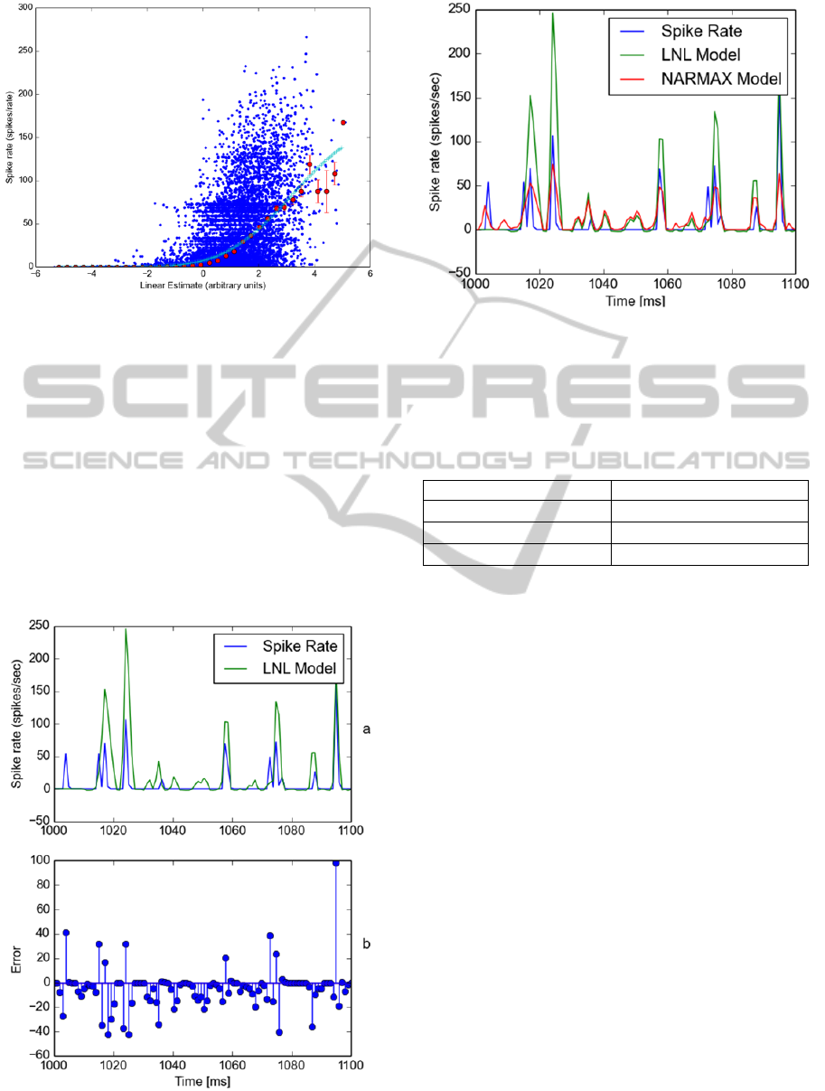
Figure 6: Nonlinearity computed for ON cell.

Figure 7 (a) illustrates the actual recorded spike rate

(blue) and the LNL model predicted spike rate

(green). Figure 7 (b) illustrates the model error. We

have also computed the RMSE as 32.29 and present

a full comparison of RMSE results in Table 1. The

RMSE results illustrate that the quadratic NARMAX

model performs best. We have also plotted the actual

neural response, LNL model predicted response and

the quadratic NARMAX model predicted response

in Figure 8 to illustrate comparative model accuracy.

Visual examination reveals the quadratic NARMAX

model has improved accuracy over the LNL model

and is comparable to the actual neural response.

Figure 7: Comparison of Linear-Nonlinear model and

actual neuron response to novel test stimulus sequence.

Figure 8: Comparative evaluation of actual spike rate,

linear nonlinear model and quadratic NARMAX model.

Table 1: Summary of RMSE for linear NARMAX,

quadratic NARMAX and Linear-Nonlinear models. The

computed RMSE values illustrate that the quadratic

NARMAX approach results in the best fitting model for

the selected dataset.

Method RMSE

Linear NARMAX

20.92

Quadratic NARMAX

18.31

Linear-Nonlinear model

32.29

5 CONCLUSIONS

Modelling biological systems is difficult due to

insufficient knowledge about the internal

components and organisation, and the complexity of

the interactions within the system. Existing

computational models of visual neurons can be

derived by quantitatively fitting particular sets of

physiological data using an input-output analysis

where a known input is given to the system and its

output is recorded as illustrated in the Linear-

Nonlinear approach in Section 4.4.

At a computational level we have presented

the use of the NARMAX system identification

technique to accurately model individual retinal

ganglion cells as shown in Section 4.2 and Section

4.3. We have presented a comparison of the actual

neuronal response and provided a comparison with

the actual neuronal response. Visual comparison

illustrates that all the methods can model the

neuronal response with accuracy although some

errors are present. Computing the RMSE provides a

more quantitative measure of error and the results

summarised in Table 1 illustrate that the quadratic

NARMAX model performs substantially better than

ModellingandAnalysisofRetinalGanglionCellsThroughSystemIdentification

163

both the LNL model and the linear NARMAX

model.

Using NARMAX system identification

techniques to express the biological input-output

coupling mathematically we have modelled highly

complex neuronal structures, and thus "identified"

ganglion cell behaviour with visual scenes. These

polynomial models represent the mapping between

perception and response. The next stage in this work

will be to increase the complexity of the stimulus by

having spatially varying stimuli; we have already

started to test the effectiveness of this using the

natural image sequences.

ACKNOWLEDGEMENTS

The research leading to these results has received

funding from the European Union Seventh

Framework Programme (FP7-ICT-2011.9.11) under

grant number [600954] (“VISUALISE"). The

experimental data contributing to this study have

been supplied by the “Sensory Processing in the

Retina" research group at the Department of

Ophthalmology, University of Göttingen as part of

the VISUALISE project.

REFERENCES

Herikstad, R., Baker, J., Lachaux, J.-P., Gray, C. M., &

Yen, S.-C. (2011). Natural Movies Evoke Spike Trains

with Low Spike Time Variability in Cat Primary

Visual Cortex. Journal of Neuroscience, 31(44),

15844-15860. doi:10.1523/JNEUROSCI.5153-10.

2011

De Boer, Kuyper, P. (1968). “Triggered Correlation”.

Biomedical ngineering, vol.BME-15, no.3, pp.169-

179. doi: 10.1109/TBME.1968.4502561 Transactions

Sakai,H.M., Naka K.I., Korenberg, M.J. (1988) "White-

noise analysis in visual neuroscience". Visual

Neuroscience, 1, pp 287-296 DOI: 10.1017

Chichilnisky EJ (2001) A simple white noise analysis of

neuronal light responses. Network 12(2):199-213.

Talebi, V., Baker, C.L. (2012). "Natural versus Synthetic

Stimuli for Estimating Receptive Field Models: A

Comparison of Predictive Robustness". The Journal of

Neuroscience, Vol. 32, No. 5., pp. 1560-1576,

doi:10.1523

Marmarelis, P.Z., Naka, K.I. (1972). White-noise analysis

of a neuron chain: An application of the wiener theory.

Science 175, 1276–1278

Victor, J., Shapley, R., Knight, B. (1977). Nonlinear

analysis of cat retinal ganglion cells in the frequency

domain. Proc. Natl. Acad. Sci. U.S.A. 74(7), 3068–

3072

Victor, J. (1979) Nonlinear systems analysis: comparison

of white noise and sum of sinusoids in a biological

system. Proc. Natl. Acad. Sci. U.S.A. 76(2), 996–998

Marmarelis, V. (2004) Nonlinear Dynamic Modeling of

Physiological Systems. Wiley Interscience, Hoboken.

Korenberg, M., Hunter, I. (1996). The identification of

nonlinear biological systems: Volterra kernel

approaches. Ann. Biomed. Eng. 24(2), 250–268.

Marmarelis VZ, Zhao X. (1997). Volterra models and

three-layer perceptions. IEEE Trans Neural Networks

8:1421.

Block-oriented Nonlinear System Identification (2010),

Lecture Notes in Control and Information Sciences,

Springer Berlin / Heidelberg, Vol. 404. Giri, F. and

Bai E.W. Eds

Nehmzow, U. (2006) Scientific Methods in Mobile

Robotics: quantitative analysis of agent behaviour.

Springer, 2006.

Ostojic S, Brunel N (2011) From Spiking Neuron Models

to Linear-Nonlinear Models. PLoS Comput Biol 7(1):

e1001056. doi:10.1371/journal.pcbi.1001056

Pillow JW, Paninski L, Uzzell VJ, Simoncelli EP,

Chichilnisky EJ. (2005). Prediction and decoding of

retinal ganglion cell responses with a probabilistic

spiking model. J Neurosci.23;25(47):11003-13.

Korenberg MJ. (1991). Parallel cascade identification and

kernel estimation for nonlinear systems. Ann Biomed

Eng 19:429.

Pillow JW, Shlens J, Paninski L, Sher A, Litke AM,

Chichilnisky EJ, Simoncelli EP. (2008) Spatio

temporal correlations and visual signaling in a

complete neuronal population. Nature 454: 995-999

Billings SA, Voon WSF. 1984. Least-squares parameter

estimation algorithms for non-linear systems. Int.J

Systems Sci 15:601.

Friederich, U., Coca, D., Billings, S.A., Juusola, M. (2009)

Data Modelling for Analysis of Adaptive Changes in

Fly Photoreceptors. Proceedings of the 16th

International Conference on Neural Information

Processing: Part I

Z. Song, S.A. Billings, D. Coca, M. Postma, R.C. Hardie,

& M. Juusola. (2009), Biophysical Modeling of a

Drosophila Photoreceptor. LNCS (ICONIP 2009, Part

I) 5863: 57–71.

Kerr, D, Nehmzow, U and Billings, S.A. (2010) Towards

Automated Code Generation for Autonomous Mobile

Robots. In: The Third Conference on Artificial

General Intelligence, Lugano. Switzerland. Atlantis

Press, Scientific Publishing, Paris, France. 5 pp.

Billings, S.A. Nonlinear system identification: NARMAX

methods in the time, frequency, and spatio-temporal

domains. John Wiley & Sons, 2013.

Lau B, Stanley GB, Dan Y (2002) Computational subunits

of visual cortical neurons revealed by artificial neural

networks. Proc Natl Acad Sci U S A 99: 8974–8979.

Prenger, R., Wu, M.C.K., David, S.V., Gallant, J.L.,

(2004) Nonlinear V1 responses to natural scenes

revealed by neural network analysis, Neural Networks,

Volume 17, Issues 5–6, Pages 663-679, 10.1016/

j.neunet.2004.03.008.

NCTA2014-InternationalConferenceonNeuralComputationTheoryandApplications

164