
Arbitrary Shape Cluster Summarization
with Gaussian Mixture Model
Elnaz Bigdeli
1
, Mahdi Mohammadi
2
, Bijan Raahemi
2
and Stan Matwin
3
1
Computer Science Department,Ottawa University, 600 king Evdard, Ottawa, Canada
2
Knowlegde Discovery and Data Mining lab, Telfelr School of Managment, University of Ottawa,
55 Laurier Ave, E. Ottawa, ON, Canada
3
Department of Computing, Dalhousie, 6050 Univeristy Ave, Halifax, Canada
Keywords: Density-based Clustering, Cluster Summarization, Gaussian Mixture Model.
Abstract: One of the main concerns in the area of arbitrary shape clustering is how to summarize clusters. An accurate
representation of clusters with arbitrary shapes is to characterize a cluster with all its members. However,
this approach is neither practical nor efficient. In many applications such as stream data mining, preserving
all samples for a long period of time in presence of thousands of incoming samples is not practical.
Moreover, in the absence of labelled data, clusters are representative of each class, and in case of arbitrary
shape clusters, finding the closest cluster to a new incoming sample using all objects of clusters is not
accurate and efficient. In this paper, we present a new algorithm to summarize arbitrary shape clusters. Our
proposed method, called SGMM, summarizes a cluster using a set of objects as core objects, then represents
each cluster with corresponding Gaussian Mixture Model (GMM). Using GMM, the closest cluster to the
new test sample is identified with low computational cost. We compared the proposed method with
ABACUS, a well-known algorithm, in terms of time, space and accuracy for both categorization and
summarization purposes. The experimental results confirm that the proposed method outperforms ABACUS
on various datasets including syntactic and real datasets.
1 INTRODUCTION
Nowadays, a large volume of data is being generated
which is even difficult to be captured and labelled. A
large volume of data is mainly generated in stream
and real time applications, in which, data is
generated rapidly, and cannot be stored bit by bit. As
a result, analysing and labelling such kind of data is
a main challenge (Guha et al., 2003)(Bifet et al.,
2009) (Charu et al., 2003). Lack of labelled data
draws attention to the application of clustering to
produce labelled data. The choice of clustering
algorithm strongly depends on data characteristic. In
small and noise free environment classical clustering
method like k-mean and k-median are commonly
used. However, in most of applications, there is no
knowledge about the number of clusters while the
shapes of clusters are non-convex and arbitrary. In
this case, density-based and grid-based clustering
methods are used. Using a clustering method that
generates arbitrary shape clusters is theoretically
ideal but the representation and analysis of each
cluster still causes many problems. For full
representation of arbitrary shape clusters, all the
samples of clusters should be preserved which is
impractical in many applications. In case of using
clustering in online applications, each cluster can be
representative of a specific pattern. These patterns
need to be kept for a long time and keeping the full
representation of the complex patterns tend to be
impractical. In this case, summarization and
extracting the key features of clusters are necessary.
Another application of clustering is categorizing the
unlabelled data. In this case, a set of clusters is
created and each cluster receives a label according to
its own samples. Each new sample is compared to
the clusters and the closest one is chosen as a cluster
that the new sample belongs to. In case of k-means,
the distance of a new sample to the centre of the
cluster is calculated, then, if the distance is less than
the radius of a cluster, new sample is attached to that
cluster. K-means and partition-based clustering
methods are sensitive to noise and cannot detect
clusters with arbitrary shape. This approach has been
43
Bigdeli E., Mohammadi M., Raahemi B. and Matwin S..
Arbitrary Shape Cluster Summarization with Gaussian Mixture Model.
DOI: 10.5220/0005071500430052
In Proceedings of the International Conference on Knowledge Discovery and Information Retrieval (KDIR-2014), pages 43-52
ISBN: 978-989-758-048-2
Copyright
c
2014 SCITEPRESS (Science and Technology Publications, Lda.)

studied in different applications but most of the
attention was towards non-arbitrary shape clustering
like k-means (Mohammadi et al., 2014)(Gaddam et
al., 2007). Arbitrary shape clustering methods
preserve all samples for each cluster and to find the
closet cluster to the new sample, distance of new
samples to all cluster members is calculated. It is
obvious that using such an approach is time
consuming. The other way to find the closet cluster
is to create a boundary for each cluster. If the new
sample is inside the boundary of a cluster then the
new sample belongs to that cluster. Finding the
boundary of arbitrary shape clusters, especially in
high dimensional problems, is a complex and time
consuming process. Moreover, it is necessary to save
too many faces to just keep borders of cluster
created by convex in higher dimension, which grows
exponentially with dimension (Kersting et al.,
2010)(Hershberger, 2009).
In this paper, we propose a new approach that fulfils
the mentioned requirements. We propose a
summarization approach to summarize arbitrary
shape clusters using Gaussian Mixture Model
(GMM). In our approach, we first find the core
objects of clusters and then we consider these core
objects as centres of GMM and represent a cluster
with a GMM. Since, GMM-based method keep all
statistical information of each cluster, it summarizes
each cluster in a way that we can use it for pattern
extraction, pattern matching, and pattern merging.
Moreover, this model is able to classify new objects.
Using GMM, each new test sample is fed into the
GMM of a cluster, and if the membership
probability to a cluster is more than a threshold, the
object is attached to that cluster.
The structure of the paper is as follows: In Section 2,
we review related work on arbitrary shape clusters
and summarization approaches. In Section 3, we
explain the general structure of the proposed
algorithm for summarization. In Section 4, we
present some discussions about the features of the
proposed method. In Section 5, we explain the
complexity of algorithm in more detail. Section 6
presents the experimental results of the proposed
algorithm in comparison with well-known
summarization algorithms. Finally, the conclusion
and future work are presented in Section 7.
2 RELATED WORK
There are various algorithms available for clustering,
which are categorized into four groups; partition-
based, hierarchical, density-based and spectral-based
clustering (Han, 2006). K-means is one of the
famous algorithms in the area of partition-based
clustering. However, using a centre and radius
makes the shape of clusters spherical which is
undesirable in many applications. In hierarchical
clustering methods such as Chameleon data is
clustered in hierarchical form but still with spherical
shape that is undesirable. Moreover, tuning the
parameters for methods like Chameleon is still
difficult (Karypis et al., 1999). Spectral clustering;
STING (Wang et al., 1997) and CLUIQE (Agrawal
et al. 1998) are able to create arbitrary shape clusters
but the major drawback of these methods is the
complexity of creating an efficient grid. The size of
grid varies for different dimensions and setting
different grid sizes and merging the grids to find
clusters are difficult. These difficulties make the
algorithm inaccurate in many cases. In the area of
arbitrary shape clustering, density-based methods
are more interesting and DBSCAN (Ester et al.,
1996) and DENCLUE (Hinneburg et al., 1998) are
the most famous ones. In density-based methods,
clusters are created using the concept of connecting
dense regions to find arbitrary shape clusters. Based
on prevalence of real time applications, there is more
interest to make these algorithms fast for streaming
applications (Guha et al., 2003)(Bifet et al.,
2009)(Charu et al., 2003).
Summarization is the solution to ease the complexity
of arbitrary shape clustering methods. The naïve
way to represent an arbitrary shape cluster is to
represent each cluster with all cluster members.
Obviously, this approach is neither practical nor
does it reflect the cluster properties. In k-means a
simple representation using a centre and radius
summarize the cluster. It is clear that this
summarization does not capture how data is
distributed in the cluster.
There are different ways to summarize arbitrary
shape clusters (Yang et al., 2011)(Cao et al.,
2006)(Chaoji et al., 2011). These algorithms use the
general idea behind the clustering methods for
arbitrary shape clusters. In the area of
summarization, the idea is to detect dense regions
and summarize the regions using core objects. Then,
a set of proper features is considered to summarize
the dense regions and their connectivity. In (Yang et
al., 2011) a grid is created for each cluster and based
on the idea of connecting dense regions, the core or
dense cells with their connections and their related
features are kept. In all summarization approaches,
these features play crucial role. In (Yang et al.,
2011) location and range of values and status
connection vector are kept however, it has some
KDIR2014-InternationalConferenceonKnowledgeDiscoveryandInformationRetrieval
44

draw backs. First, creating grids on each cluster is
time consuming. Second, considering all grids needs
spending a lot of time and space which is impractical
in many cases. Cao et al. (Cao et al., 2006) use the
idea of finding core objects to generate the cluster
summery. The most significant drawback of this
work is that the number of core objects is large and
in some cases, it is equal to the number of input
samples. Moreover, a fixed radius specifies the
neighbourhood that does not represent the
distribution of objects in each cluster (Cao et al.,
2006). Chaoji et al. represent a density-based
clustering algorithm named ABACUS for creating
arbitrary shape clusters (Chaoji et al., 2011). The
summarization part in their approach is based on
finding the core objects and the relative variance
around the objects. In most of arbitrary shape
clustering methods, we need two parameters;
number of neighbours and a radius. The most
interesting and noticeable part in Chaoji et al. work
is that the number of neighbours is the only
parameter for their algorithm and they generate
radius using data distribution. The significant
drawback in their work is that the algorithm may
generate many core points.
In all above mentioned summarization approach,
focus is on preserving the cluster members and they
don’t consider any usage of clustering for
classification purpose. Clustering approaches are
created to summarize data and categorized the input
data into some groups, but it can also be used as a
pre-processing phase of classification task (Ester,
1996)(Hinneburg, 1998). Each cluster has a label
and for each new object the closest cluster is found
and the object gets the label of that cluster. The
mentioned approaches like k-means summarize the
clusters, but they still consider the concept of circles
around the core objects to find the closest cluster
which is inaccurate. Graph-based structures are more
accurate but they are time consuming. Anomaly
detection is one of the applications of clustering in
classification (HE, 2003)(Borah and Bhattacharyya,
2008)(Gaddam, 2007)(Mohammadi, 2014). In this
area, those objects which are outside of cluster
boundaries are considered as anomaly. In previous
works, clusters are generated using k-means and
summarized with a centre and a radius which is
inaccurate.
In this paper, we present an approach to summarize
clusters using Gaussian Mixture Models. Our
approach covers both areas; it is a good
representative of a cluster and it can be used for
classification purpose.
3 GENERAL STRUCTURE OF
THE SGMM ALGORITHM
The main idea behind the density-based clustering
algorithms is to connect dense regions to create a
cluster. With this idea, a set of core objects are
detected and they are connected to each other using
the shared neighbourhood.
DEFINITION 3.1. In dataset D for a given k and
radius r, an object
is a core object if
∀x ∈ D, o
∈Cdo
,
,xk
Where C is set of core objects and (
‖
‖
shows the
number of objects with distance less than r from the
core object. Detection of k and r is critical in
identifying good clusters.
Figure 1: Structure of the SGMM method for cluster summarization.
The
original
Cluster
Finding
Core
Points
Feature
Extractio
n
Absorptio
n
GMM
Extractio
n
,Σ
,
,Σ
,
,Σ
,
,Σ
,
,Σ
,
ArbitraryShapeClusterSummarizationwithGaussianMixtureModel
45

The concept of core objects has been used to
generate the backbone of a cluster and generate
summery of the cluster. In some recent works
(Chaoji, 2011) using a given k and core objects idea,
they detect the backbone of cluster. In this paper, we
use the same idea but with more concentration on
decreasing the number of core objects and the time
of detection of these core objects. The general idea
for summarization of each cluster in this paper is
based on Gaussian Mixture Model. Since Gaussian
Mixture Model preserves the distribution of data
using a set of Normal Distributions, it is a good
candidate for summarizing any cluster. Therefore,
we can apply simply EM algorithm on each cluster
to find its GMM representative, but the main
concern is to find the number of GMM components.
In our proposed approach, we first find the number
of GMM components, and then we find appropriate
GMM for each cluster. Our method, Summarization
Based on Gaussian Mixture Model (SGMM), has
four main steps that are depicted in Figure 1. First, a
set of objects called core objects are detected. These
objects are representative of a cluster and can
generate the original cluster as needed. After
detection of backbone objects, there comes the
absorption step, where the objects attached to the
core object are absorbed and represented by core
objects. Then by introducing a new feature set for
each object, cluster is summarized while its original
distribution is preserved. Finally, each cluster is
presented as a GMM. In the following sections, we
describe each step in more detail.
3.1 Finding Core Objects
In this step, we find the core objects that create the
backbone of each cluster. There are different ways to
find the core objects in each cluster, but time is the
main concern in this case. In this step, we consider a
radius based on which we find the neighbours for all
objects for each cluster. Then we sort all objects
based on the number of neighbours. The first core
object is the one with the maximum number of
neighbours. All the neighbours of this object are
removed from the list of possible core objects. With
this approach, we reduce the overlap of core objects
as much as possible. Among the remaining objects,
we find the next objects with maximum number of
neighbours. We label this object as a core object and
remove neighbours of this object from further
consideration. In this way with a heuristic approach,
we find the core objects located in dense regions and
all parts of cluster are covered using them. The new
definition of the core objects with our methodology
is presented as follow.
DEFINITION 3.1.1. (Core Object) A core object is
the object that has the maximum number of
neighbours in comparison with other objects in its
neighbourhood. The core object is not in the
neighbourhood of another core object.
∀c
∈Cij,dc
,c
r
Where i and j are the index for different core points
and d refers to the distance of two objects.
3.2 Absorption and Cluster Feature
Extraction
The goal of summarization is to find a good
representative of each cluster and core objects are
the only objects that we preserve in each cluster
while the rest of the objects in the cluster are
removed. After finding all core objects in each
cluster, the next step is to define a cluster using core
objects. It is obvious that considering only core
objects cannot be a good representative of each
cluster. The core objects have to be accompanied
with a set of features related to the cluster to
represent a cluster. This is why we define a set of
features for each core object which are good
representative for distribution around each core
object.
DEFINITION 3.2.1: (Core Object Feature) (CF)
Each core object is represented by a triple
〈
,
,
〉
.
In this definition
is the core object and Σ
is the
covariance calculated using the core object and all
objects in its neighbourhood.
/ is the
weight of core object, n is the number of objects in
the neighbourhood of core object
, and CS is
cluster size.
shows the proportion of objects
which are in the neighbourhood of the core object.
Using the features for each core object, we estimate
samples scattering around each core object without
keeping the entire samples in the neighbourhood.
3.3 GMM Representation of Clusters
After finding the core objects and all necessary
features for each cluster, we generate a Gaussian
Mixture Model for each cluster.
DEFINITION 3.3.1. A Gaussian Mixture Model is a
combination of a set of normal distributions. Given
KDIR2014-InternationalConferenceonKnowledgeDiscoveryandInformationRetrieval
46
feature space ⊂
, a Gaussian Mixture Model
: → with n component is defined as:
)()(
1
xwxg
ii
n
i
i
T
iii
ii
xx
i
d
ex
)()(
2
1
1
)2(
1
)(
(1)
Based on all
, 1 ⋯ , a GMM is defined
over a cluster. Each component for GMM is created
using a core object, its covariance and the weights.
In the formula in equation (1), μ
is the centre of the
i
th
GMM component, which is set to the coordination
of core object and therefore, μ
c
. The covariance
is set to covariance of i
th
core object covariance, that
is Σ
. The weight for each component is the weight
of core object and as a result w
in the equation (1) is
set to the weight of core object c
which is ω
.
The main goal of cluster summarization is to present
a cluster in a way that it keeps the overall
distribution of the cluster while reducing the number
of objects in the cluster which is critical in stream
data mining and online environment. To use a
cluster as a class in classification, we need to find
the closest cluster to a new incoming sample. In an
arbitrary shape cluster, all objects represent a cluster
and to find a right cluster for a new sample, it has to
be compared with all objects in a cluster. GMM-
based summarization fulfils both requirements for
both applications; summarize data for the real time
applications; generate a proper representation for
each cluster to use them in classification approach.
4 GAUSSIAN MIXTURE
SUMMARIZATION
As each GMM consists of a set of Gaussian
distributions, finding the number of GMM
components is a challenging issue. In this paper, we
proposed a solution to calculate number of
components for each cluster by finding the core
points. In our approach, number of components for
GMM is set to the number of core objects in a
cluster.
There are two essential features that should be
considered. Each summarization technique has to
preserve the original shape and the distribution of
the data. Summarization of data using GMM has
both characteristics. In SGMM some objects are
selected in a way that they follow the general
structure of data. Not only finding the core object is
easy and fast but also it still follows the shape of the
cluster. The algorithm starts from dense regions in
the cluster and then goes to the most scattered part
with consideration of covering all data objects in the
cluster. In the SGMM method, the core objects are
the ones which are in the center of dense regions and
they cover all data. Therefore, for each region a
representative object is chosen and then collection of
these representative objects presents the entire
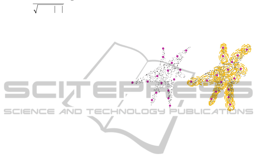
cluster. Figure 2, shows the core objects generated
for a cluster. This figure shows that the generated
core objects follow the general structure of the
cluster.
Figure 2: Cluster with the core objects.
Finding the general structure of a cluster using a set
of objects is not enough for achieving high accuracy
in classification applications. In many applications,
we would like to keep the original or summery of
data for more detail investigation. Saving the core
objects cannot reveal any information about the
distribution of data. Therefore, we need to find
distribution information around the core objects and
as we mentioned above, we capture such
information using the covariance around core
objects. Using such information, we are able to
regenerate the original data.
Finally, we need to know the contribution of each
core object in generation of data. We find out the
weight of each core object based on the number of
neighbours that each object has. With knowing the
location of core objects, related covariance and the
weights, we summarize data using a GMM with the
minimum loss of information. The relative GMM for
a cluster is depicted using contour plots in Figure 2.
5 COMPUTATIONAL
COMPLEXITY
In stream data mining application, using a fast
algorithm is a critical requirement. In this section,
we examine the computational complexity of the
proposed algorithm.
ArbitraryShapeClusterSummarizationwithGaussianMixtureModel
47
In the first step of algorithm, we find the neighbours
of each object; with N as the number of objects it
takes
O(
)
to find neighbours. Then, we need to
sort the objects and absorb neighbours of the core
objects that takes O(NlogN). In absorbing step, we
find the number of neighbours for each core object
and its related variance. We consider O(NlogN) for
the second part of the proposed method which is the
worst case.
So, the final complexity of the proposed algorithm is
O(
)
. In the grid-based method a
considerable amount of time is spent to create the
grid and further investigation to find core grids and
connecting them. In some other density-based
methods such as ABACUS there are iterations to
find core objects and to reallocate them which are
time consuming. The output of SGMM is almost the
same as that of ABACUS but the proposed method
is not time consuming in comparison to ABACUS.
The experiment results show that our heuristic leads
to the same result with one step. In the next section,
we develop a comparison between the required time
of our method and the one for ABACUS. The results
illustrate that the proposed method outperforms
ABACUS in term of time.
6 EXPERIMENTAL RESULTS
We use both synthetic data set and the real data set
in our experiments. Time and space complexity and
the goodness of clustering are three different criteria
that we evaluate our algorithm based on. Moreover,
we set up different experiments to see the efficiency
of our algorithm for categorizing new samples. We
compared our algorithms with ABACUS (Chaoji,
2011) which is one of the well-known
summarization methods in literatures. All
experimental results are generated in Matlab running
on a machine with Intel CPU 3.4 GHz and 4GB
memory.
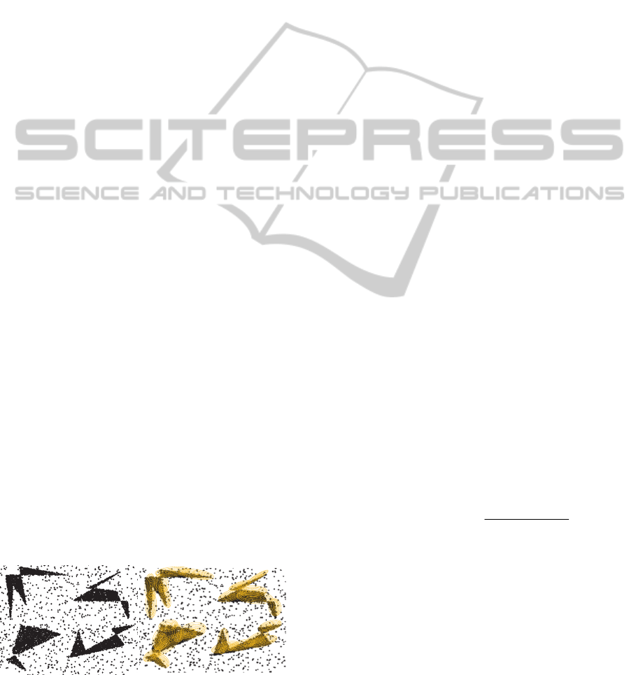
The first data set is a synthetic dataset as shown in
Figure (3). We use this dataset to visualize the
effectiveness of the proposed algorithm.
Figure 3: Synthetic data with related GMMs.
This figure shows 4 clusters and set of objects used
in testing phase. In this Figure we see each cluster is
represented by a GMM depicted with a contour plot.
KDD dataset and some other UCI datasets are
considered in our experiments to evaluate the
accuracy of our algorithm on some real datasets.
6.1 Clustering Goodness
To show the efficiency of SGMM method, we set up
experiments in which we summarize the dataset
using core objects then we used these core objects
and their related variance and weights to regenerate
the dataset. The difference between the first dataset
and regenerated dataset by core objects shows the
strength of summarization algorithm. Experimental
results show that SGMM method summarize dataset
better than ABACUS method. To visualize the
results, we generated a synthetic data with four
clusters. Figure 4 from left to right shows the
original dataset, core objects of each cluster and the
dataset set regenerated using core objects using
ABACUS and SGMM method. This figure shows
that the core objects follow the original structure of
the clusters and the regenerated clusters are similar
to the original ones. This figure depicts the ability of
SGMM method, and it shows that the summery
generated by SGMM regenerates the original dataset
better in comparison to ABACUS method. The
difference between the accuracy of summarization
of ABACUS and SGMM is clearer in the cluster
with star shape. SGMM summery regenerate the
data with star shape, but ABACUS method could not
regenerate the same shape. These figures are just for
visualization the result and to show the efficiency of
the algorithm, we use Dunn and DB index.
The Dunn index (Dunn, 1979) is a validity index
which identifies compact and well-separated classes
defined by equation (2) for a specific number of
classes:
1,..., 1,...,
1,...,
(, )
min min
max ( )
ij
nc
incjinc
k
knc
dist c c
D
diam c
Where nc is the number of classes, and dist(c
i
,c
j
) is
the dissimilarity function between two classes C
i
and
C
j
. The large values of the index indicate the
presence of compact and well-separated classes. In
our experiments, we first calculate the Dunn index
for the original datasets. Then, summarize the
dataset and re-generate the data again using the final
core objects of GMMs and we find out the Dunn
index for regenerated data. Finally, we get the
difference between Dunn index of original dataset
(2)
KDIR2014-InternationalConferenceonKnowledgeDiscoveryandInformationRetrieval
48
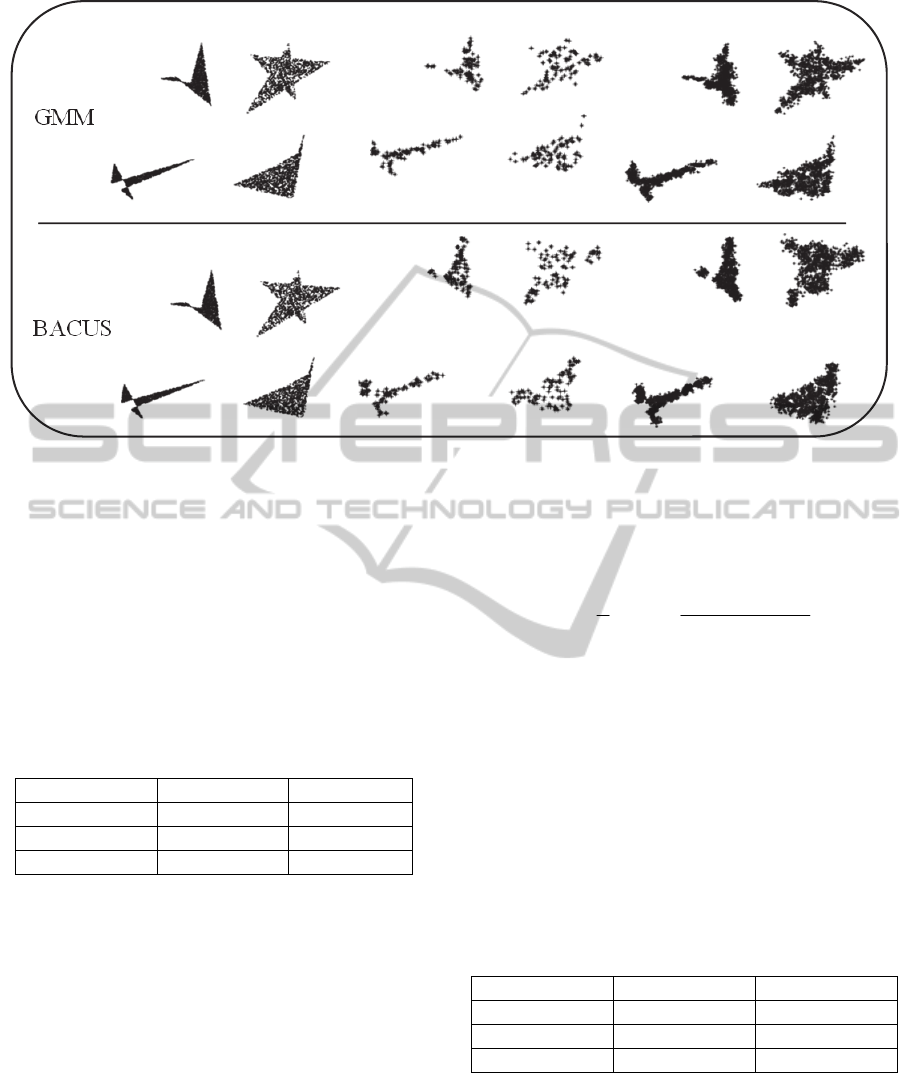
Figure 4: The first dataset is the original dataset, the second one is the core points and the third one is regenerated dataset
using the core points based on ABACUS and SGMM methods.
and the one which is regenerated. Using this
experiment, we want to evaluate the regeneration
ability of the SGMM method. In other words, we
want to show how the SGMM method regenerates
the data which follows the shape and distribution of
the original data. Table 1 shows the results of this
experiment. Each value in this table is the average of
30 independent runs.
Table 1: Difference of Dunn Index for original and
regenerated dataset.
Dataset\Index SGMM ABACUS
Synthetic Data
0.02358 0.076932
KDD
0.027701 0.034321
Segment
0.008841 0.014636
The closer the value to zero, the better the result we
get. Based on the difference of Dunn index table,
SGMM always outperforms ABACUS by far. For
example in case of Segment dataset, the difference
between the dataset generated by SGMM and the
original dataset is almost zero while this value for
ABCUS is around 0.01. This experiment illustrated
that SGMM follow the sample distribution of the
original dataset better than ABACUS. The next step
is to repeat the experiment using DB cluster index.
The second measurement we used is DB index
(Davies and Bouldin, 1979) which is a function of
the ratio of the sum of within cluster scatter to
between-cluster separation. DB index is defined as
in equation (3).
n
i
jin
jnin
ji
QQS
QSQS
n
DB
1
),(
)()(
max
1
(3)
n is the number of clusters,
is the average
distance of all objects of the cluster to their cluster
centre, and
,
is the distance between clusters
centres. Hence, the ratio is small if the clusters are
compact and far from each other. Consequently,
Davies-Bouldin index will have a small value for a
good clustering. As what we did for Dunn index, we
find the distance of the original and regenerated
data. Table 2 shows the experimental results of DB
index on different datasets.
Table 2: Difference of DB Index for original and
regenerated dataset.
Dataset\Index SGMM ABACUS
Synthetic Data
0.006638 0.017609
KDD
0.195763 0.232498
Segment
0.0429764 0.0546819
Result based on Dunn and DB index shows that the
SGMM method generates more accurate summery
of dataset and in case of regenerating the original
dataset SGMM follows the original pattern better.
Original Dataset Core points Regenerated Dataset
SGMM
ABACUS
ArbitraryShapeClusterSummarizationwithGaussianMixtureModel
49
6.2 Clustering Accuracy
As mentioned above, clustering is used in
classification as a preprocessing step. The
application we focused on, in this part, is anomaly
detection. We first cluster the normal data into some
clusters then we consider these clusters as normal
behaviours. The membership probability for each
new sample is calculated. If the sample belongs to a
cluster, it is normal otherwise it is an attack. For this
purpose, we consider KDD dataset and we find out
the accuracy of attack detection. Using GMM in
classification is our proposed method and to the
knowledge of author there is no other work similar
to our approach. The only approach that has been
used in an arbitrary shape cluster to label new
sample is to consider all member of clusters which is
the Naïve approach. In our experiment, we created
GMM using our set of core objects and ABACUS
core objects. As we mentioned, we created the core
objects using a simple method that spends less time
and space. Therefore, there can be a doubt about the
accuracy of categorizing using the clusters using our
method? The experiment shows that our approach
does not decrease the accuracy.
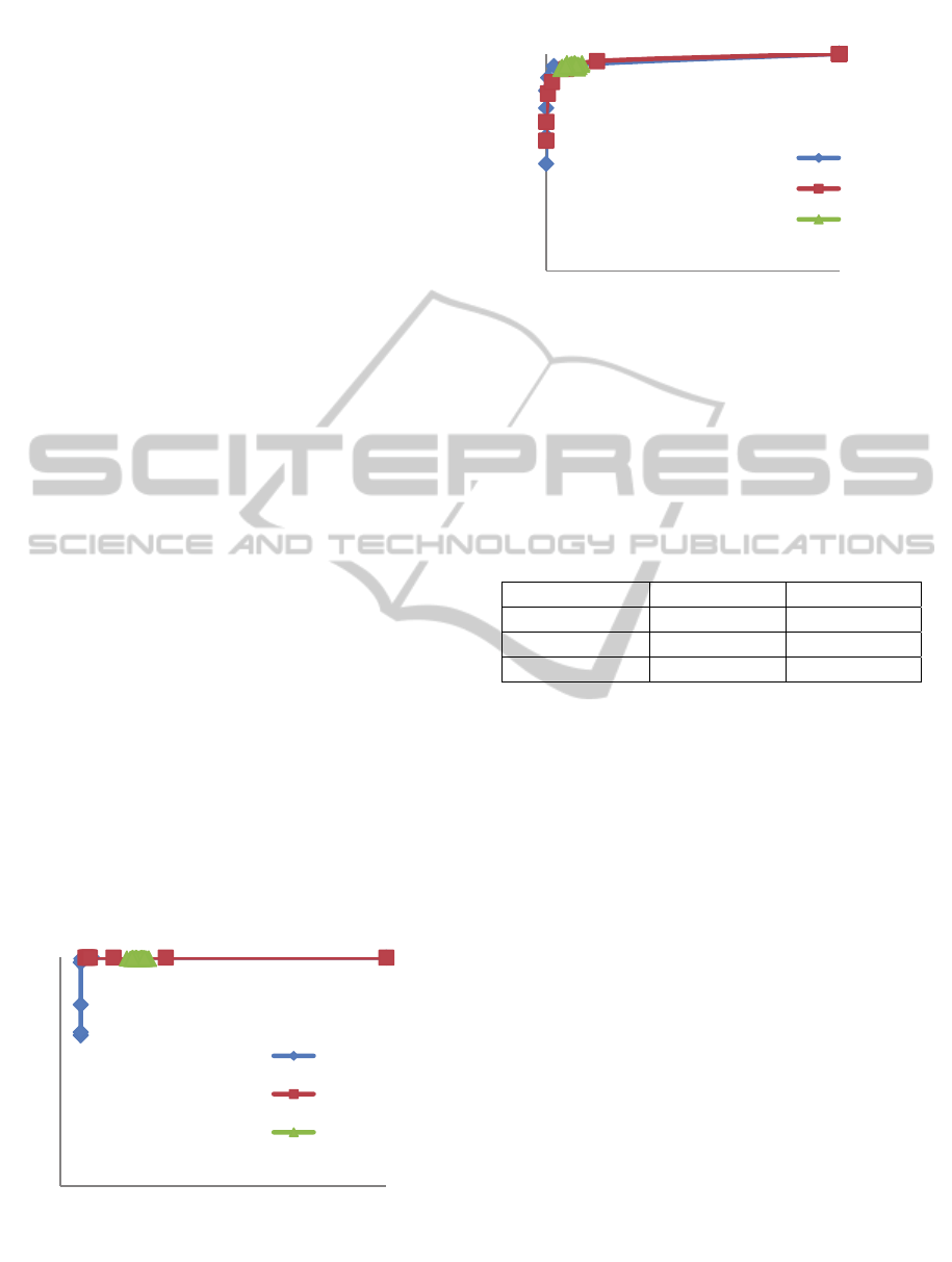
The ROC curve based on detection rate and false
alarm rate for KDD dataset depicted in Figure 5. It
shows while the ABACUS is more time consuming
and find out too many core objects our method has
the same and sometimes better accuracy. Figure 6
shows the result for synthetic dataset. It shows that
the accuracy of our approach is better than Naïve
and ABACUS method. The result for synthetic
dataset set shows that in spite of using clustering in
categorizing new objects the accuracy is still good
and comparable to the accuracy of classification
methods.
Figure 5: ROC curve for KDD dataset.
Figure 6: ROC curve for Synthetic dataset.
Table 3 shows more results on some other datasets,
which confirms that summarizing and clustering
data using SGMM method outperforms ABACUS
method. The first value in Table 4 is the false alarm
rate and the second one is the detection rate.
Table 3: Accuracy of SGMM and ABACUS method in
anomaly detection.
Dataset\Index SGMM ABACUS
Synthetic Data
(2,94) (1.9,87)
KDD
(6.301, 100) (9.041, 100)
Segment
(33.83,94.39) (32.82,94.54)
6.3 Algorithm Complexity
Two main concerns in the area of summarization are
the time spent to find the summery of a cluster and
the number of objects preserved for it. Table (4)
shows the space and the time spent to find the
summery of a cluster for different datasets. This
table shows that SGMM decreases time and space to
summarize each cluster. It is clear that SGMM
method uses only one iteration to find core objects
while ABACUS method runs many iterations to find
out the core objects and therefore, SGMM is faster.
On the other side, SGMM summarizes cluster with
less number of core objects. The reason lies in the
SGMM algorithm in finding core objects. If an
object is core object, all objects in its neighborhood
are removed from possible set of core objects and
we do not consider them. In this case, we are able to
decrease the time and space complexity both. Table
4 and 5 shows the time and space used by SGMM
and ABACUS and it shows that using SGMM we
decrease time and space considerably.
90
91
92
93
94
95
96
97
98
99
100
0 20406080100
Detection Rate
False Alaram Rate
KDD
SGMM
ABACUS
Naïve Approach
0
10
20
30
40
50
60
70
80
90
100
0 20406080100
Detection Rate
False Alarm
Synthetic data
SGMM
ABACUS
Naive
KDIR2014-InternationalConferenceonKnowledgeDiscoveryandInformationRetrieval
50
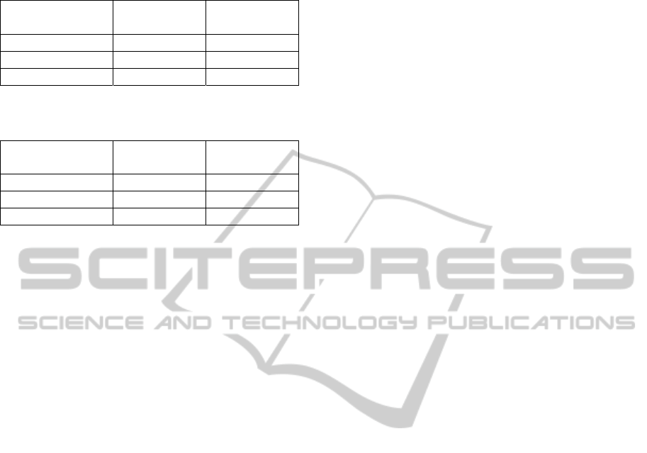
Table 4: Number of core objects for ABACUS and
SGMM methods.
Dataset\Space
complexity
SGMM ABACUS
Synthetic Data 51 120
KDD 46 272
Segment 52 55
Table 5: The time complexity for ABACUS and SGMM
methods.
Dataset\Time
complexity
SGMM ABACUS
Synthetic Data 388 sec 1261 sec
KDD 222 sec 836 sec
Segment 7 sec 19 sec
7 CONCLUSIONS
In this paper, we presented a new approach for
summarizing the arbitrary shape clusters. Our
proposed algorithm, named SGMM, represents each
cluster by a Gaussian Mixture Model (GMM) using
sets of core objects. Each GMM is a representative
of the distribution of whole members in a cluster.
Moreover, SGMM is able to find the closest cluster
for each new incoming sample. The experimental
results based on Dunn and DB index confirms that
the distribution of clusters is preserved after
summarization. Additionally, in case of
classification, the accuracy using SGMM is
acceptable. Our proposed algorithm also exhibits a
low computational cost which makes it a suitable
approach for clustering stream data. Extending the
density based clustering to make it faster is a part of
our future work.
REFERENCES
Agrawal, J. Gehrke, D. Gunopulos, and P. Raghavan,
1998, “Automatic sub-space clustering of high
dimensional data for data mining applications,”
SIGMOD Rec, vol. 27, pp.94–105.
Bifet, A, Holmes G, Pfahringer B 2009. New ensemble
methods for evolving data streams. In: Proceedings
ofthe 15th ACM SIGKDD international conference on
knowledge discovery and data mining. pp 139–148.
Borah B., Bhattacharyya D., 2008. Catsub: a technique for
clustering categorical data based on subspace. J
Comput Sci2:7–20.
Charu C. Aggarwal , T. J. Watson , Resch Ctr , Jiawei Han
, Jianyong Wang , Philip S. Yu, 2003, A framework
for clustering evolving data streams. Proceedings of
the 29th VLDB Conference, Berlin, German.
Davies D.L.,. Bouldin D.W. A cluster separation measure.
1979. IEEE Trans. Pattern Anal. Machine Intell. 1 (4).
Pp. 224-227.
Yang D, Elke A, , Matthew O. Ward. 2011,
Summarization and Matching of Density-Based
Clusters in Streaming Environments. Proceedings of
the VLDB Endowment (PVLDB), Vol. 5, No. 2, pp.
121-132.
Ester. M., Kriegel. H., Sander. J., and Xu. X. 1996, A
density-based algorithm for discovering clusters in
large spatial databases with noise. In KDD, pages
226–231.
Cao F, Ester M, Qian W, Zhou A, Density-based, 2006,
clustering over an evolving data stream with noise. In
2006 SIAM Conference on Data Mining. 328—339.
G. Karypis, E.-H. Han and V. Kumar, 1999, Chameleon:
Hierarchical Clustering Using Dynamic Modeling,
Computer, 32:8, pp. 68–75.
Gaddam S, Phoha V, Balagani K., 2007, K-means+id3: a
novel method for supervised anomaly detection by
cascading k-means clustering and id3 decision tree
learning methods. IEEE Trans Knowl Data Eng
19(3):345–354.
Guha S, Meyerson A, Mishra N et al, 2003, Clustering
data streams: theory and practice. IEEE Trans Knowl
Data Eng 15(3):505–528.
Han. J, Kamber. M, J. Pei. 2006. Data Mining: Concepts
and Techniques, Third Edition (The Morgan
Kaufmann Series in Data Management Systems).
HE, Z., XU, X., AND DENG, S. 2003. Discovering
cluster-based local outliers. Pattern Recog. Lett. 24, 9–
10,1641–1650.
Hinneburg. A. and Keim. D. A. 1998. An efficient
approach to clustering in large multimedia databases
with noise,” in KDD , , pp. 58–65.
John Hershberger, Nisheeth Shrivastava, Subhash Suri,
2009. Summarizing Spatial Data Streams Using
ClusterHulls, Journal of Experimental Algorithmics
(JEA), Volume 13,. Article No. 4 ACM New York,
NY, USA.
K. Dunn, j. Dunn. Well separated clusters and optimal
fuzzy partitions. Journal of Cybernetics ,(4), (1974),
pp. 95-104.
Kristian Kersting, Mirwaes Wahabzada, Christian
Thurau, Christian Bauckhage., 2010. Hierarchical
Convex NMF for Clustering Massive Data. ACML:
253-268.
Mohammadi M, Akbari A, Raahemi B, Nasersharif B,
Asgharian H. 2014. A fast anomaly detection system
using probabilistic artificial immune algorithm capable
of learning new attacks. Evolutionary Intelligence
6(3): 135-156.
Chaoji V, Li W, Yildirim H, Zaki M, 2011. ABACUS:
Mining Arbitrary Shaped Clusters from Large
Datasets based on Backbone Identi
fication. SDM,
page 295-306. SIAM / Omnipress,.
Wang. W., Yang. J., and Muntz. R. R., 1997. Sting: A
statistical information grid approach to spatial data
ArbitraryShapeClusterSummarizationwithGaussianMixtureModel
51

mining. In Proceedings of the 23rd International
Conference on Very Large Data Bases ,ser.VLDB’97.
San Francisco, CA, USA:Morgan Kaufmann
Publishers Inc., pp.
KDIR2014-InternationalConferenceonKnowledgeDiscoveryandInformationRetrieval
52
