
Where Did I(T) Put It?
A Holistic Solution to the Automatic Construction of Topic Trees for Navigation
Hans Friedrich Witschel, Barbara Thönssen and Jonas Lutz
Fachhochschule Nordwestschweiz, Olten, Switzerland
Keywords: Information Management, Clustering, Topic Tree Induction, Cluster Labeling.
Abstract: Managing information based on hierarchical structures is prevailing, be it by storing documents physically
in a file structure like MS explorer or virtually in topic trees as in many web applications. The problem is
that the structure evolves over time, created individually and hence reflecting individual opinions of how
information objects should be grouped. This leads to time consuming searches and error prone retrieval
results since relevant documents might be stored elsewhere. Our approach aims at solving the problem by
replacing or complementing the manually created navigation structures by automatically created ones. We
consider existing approaches for clustering and labelling and focus on yet unrewarding aspects like having
information objects in inner nodes (as it is common in folder hierarchies) and cognitively adequate labelling
for textual and non-textual resources. Evaluation was done by knowledge experts based on a comparison of
retrieval time for finding given documents in manually and automatic generated information structures and
showed the advantage of automatically created topic trees.
1 INTRODUCTION
Hierarchical structures of information are prevailing
but inefficient for locating information if they
become too large (Bruls et al. 2000). The problem is
exacerbated if the hierarchical structure emerges
unsupervised and is created individually reflecting
personal opinions on how information objects
should be grouped – not necessarily shared by
others. This leads to time consuming search and
error prone retrieval results: one might find the
document searched for – but how to be sure that a
later version isn’t stored elsewhere?
In our work we investigate if the manually
created hierarchies can be replaced – or
complemented – by automatically created structures
in order to reduce time for searching and to increase
the recall and precision. Our hypothesis is that
information is found much quicker navigating in an
automatically created structure since its grouping of
information is impartial based on automatic
clustering.
Our work considers existing approaches for
clustering and labelling but focusses on yet
unrewarding aspects like cognitively adequate
labelling for textual and non-textual resources. The
research was carried out within the SEEK!sem
project, funded by the Swiss Confederation
(Commission for Technology and Innovation CTI.
Project no 14604.1 PFES-ES). The work
complements previous work on automatically
identifying related information objects regardless of
their format (Lutz et al. 2013). Evaluation was done
by knowledge experts based on a comparison of
retrieval time for finding given documents in
manually and automatic generated information
structures.
2 APPLICATION SCENARIO
The SEEK!sem project is a Swiss national funded
research project . Business partner in the project
is a Swiss software vendor who offers a web-
based information management system called
SEEK!SDM (http://www.bdh.ch/datamanagement/
seeksdm.html). Electronic documents (i.e. text but
also images) can be uploaded into an Enterprise
Portal and filed manually into folders. When
SEEK!SDM is installed the folder structure is
empty, i.e. consists of a root node only. Building up
the hierarchical structure as well as defining tags for
classifying information objects is to be done
manually. As described by (Thönssen 2013) in
194
Friedrich Witschel H., Thönssen B. and Lutz J..
Where Did I(T) Put It? - A Holistic Solution to the Automatic Construction of Topic Trees for Navigation.
DOI: 10.5220/0005075201940202
In Proceedings of the International Conference on Knowledge Management and Information Sharing (KMIS-2014), pages 194-202
ISBN: 978-989-758-050-5
Copyright
c
2014 SCITEPRESS (Science and Technology Publications, Lda.)

general, if any then no more than the upper two to
three levels of such structures are defined on
company level, for example organized by products,
clients or temporal aspects. All deeper structures are
created individually leading to the well-known
problems of incomprehensible folder structure and
hence long search times and the danger of missing of
relevant information. The SEEK!SDM system
allows for storing information resources on all
nodes.
These resources are folders, called ‘dossiers’
containing the actual information objects which
might be of various formats, e.g. text, image but also
personal or organisational data. The topics (nodes)
of the topic tree, the dossiers and the structure of the
dossiers are created manually guided by personal
opinions.
Hence, different versions of the same
information object but also the very same
information object might be stored in different
dossiers (and different nodes) increasing the
problem of finding all relevant information objects.
Searching for information is time consuming;
adding the risk of not finding relevant documents at
all or finding the relevant but not the latest document
provides the motivation for coming up with a
hierarchical structure of information which is (a)
independent from personal opinions and (b)
complete with respect to filing related information
objects (e.g. all versions, all formats of a document)
in the same node.
Rather than searching blindly in inexplicable
hierarchical structures, always uncertain if the right
information object has been found, search in an
objectively comprehensible structure may decrease
retrieval time and the risk of not finding everything.
With our approach of automatically clustering
information objects, we provide such an objectively
comprehensible structure.
3 RELATED WORK
3.1 Hierarchical Clustering of
Documents
Hierarchical agglomerative clustering (HAC) (Cios
et al. 1998) is a very well-known and popular
method for grouping data objects by similarity. HAC
is initialized by assigning each object to its own
cluster and then, in each iteration, merging the two
most similar clusters into a new cluster. This
procedure results in a so-called dendogram, a binary
tree of clusters where each branching reflects the
fact that two child nodes were merged to a parent
node in a given iteration of the algorithm.
When the data objects are documents, a
dendogram can be used as a means of navigation
within a document collection (see e.g. (Alfred et al.
2014)).
Alternative hierarchical clustering methods have
also been proposed for navigation, e.g. scatter/gather
(Cutting et al. 1993), where the user can influence
the clustering through interaction at run-time.
It has been recognized by many researchers that
binary trees are not an adequate representation of the
similarities and latent hierarchical relationships
between elements and clusters (Blundell et al. 2010).
Therefore, a number of approaches have been
proposed that cluster elements into multi-way trees.
Many of these approaches come from the area of
probabilistic latent semantic analysis, e.g. based on
Latent Dirichlet processes (Zavitsanos et al. 2011).
Other probabilistic approaches are based on greedy
algorithms, e.g. Bayesian Rose Trees (Blundell et al.
2010).
Another approach, similar to ours, uses a
partitioning of the dendogram resulting from HAC
to derive a non-binary tree (Chuang & Chien 2004).
In this approach, for a current (sub-)tree, an optimal
cut level for the corresponding dendogram is chosen
in a way that maximizes the coherence and
minimizes the overlap of the resulting clusters.
Then, this procedure is applied to the (binary) sub-
trees of the resulting clusters. The approach has been
shown to be effective, but it has a number of free
parameters that are hard to understand for end users.
It is a problem of all these approaches that data
elements are not allowed to reside within inner
nodes of the tree – something that users usually
expect and that will happen when hierarchies are
created manually.
3.2 Learning Topic Trees
Hierarchical structures for organizing document
collections only become useful when each node in
such a structure has a meaningful label – only then it
is possible for users to navigate and locate desired
content. We call a hierarchical organization of
documents (a tree) a topic tree if the nodes of the
tree have labels.
A number of researchers have explored the
challenge of labeling clusters in a flat (i.e. non-
hierarchical) clustering of textual documents
(Popescul & Ungar 2000), (Radev et al. 2004),
(Muller et al. 1999). These approaches are based on
term frequency statistics, selecting descriptors that
WhereDidI(T)PutIt?-AHolisticSolutiontotheAutomaticConstructionofTopicTreesforNavigation
195

are both representative for a given cluster and
discriminative w.r.t. the other clusters.
However, as will be argued below, labeling
hierarchical clusterings is a task with additional
challenges, e.g. the desire to avoid redundancies in
labels between parent and child nodes of the
hierarchy.
Learning to organize natural language terms
hierarchically out of text (often termed taxonomy or
ontology learning, see e.g. (Caraballo 1999)) is a
topic that is closely related to labeling topic trees,
and that has received much research attention. It has
also been explicitly related to hierarchical document
structures, see e.g. (Lawrie et al. 2001),(Glover et al.
2002).
There is considerably less research on how to
label hierarchical clusterings. The work in
(Treeratpituk & Callan 2006), as a notable example
of such research, focuses on providing cluster labels
based on term frequency distributions such that
labels both summarise a cluster and help to
differentiate it from its parent and sibling nodes.
4 RESEARCH QUESTIONS AND
METHODOLOGY
4.1 Research Questions
Our contribution is a holistic solution to building a
topic tree, in which we address the following, yet
unanswered research questions that arise when
applying clustering techniques to topic tree
induction in practice:
- How can a topic tree be built in such a way
that it naturally allows data elements to
reside within inner nodes of the tree? In most
practical applications of topic trees - consider
for instance a folder hierarchy in a file system –
inner nodes can contain data elements. This is
not possible in any of the above-mentioned
approaches where data elements can only reside
in the leaves.
- How can a hierarchy of clusters be labelled in
a cognitively adequate way? The labels of the
topic tree nodes are crucial for orientation of the
navigating user. Yet, labeling a hierarchical set
of clusters is fundamentally different from
labeling a flat clustering. That is because
redundancy needs to be avoided: a parent
node’s label should only refer to those
characteristics that are shared among all of the
child nodes. And, even more importantly and to
avoid redundant information while browsing a
tree from the root towards the leaves, each child
node should be labeled using only those
characteristics that discriminate it from the
others and from its parent.
-
How to enable such labeling not only for
textual documents, but also other kinds of
resources (e.g. images or persons)? In real-life
applications, the elements to be clustered are not
only text, but can be multimedia elements,
contacts (i.e. persons) etc. Most existing cluster
labeling approaches work only for text. What
adaptations are needed for labeling
corresponding clusters?
4.2 Research Methodology
We will propose a new algorithm for topic tree
induction that works on textual documents, but also
other kind of resources and that results in a non-
binary tree with labeled nodes.
We will explore two labeling methods: one
results directly from a new concept (“similarity
explanation”) introduced as part of the new
clustering algorithm. The other is an adaptation of a
classical frequency-based cluster description method
for the case of arbitrary (i.e. possibly non-textual)
resources and for the purpose of avoiding
redundancy of cluster descriptions.
Our evaluation will be based on an experiment
where test persons have to search for a given file
within several versions of a topic tree. The time
needed to locate the file will be used as an indication
of the cognitive adequacy of the tree representation.
This is fundamentally different from the
evaluation methodologies used in previous work,
most of which used a gold standard topic tree and
measured the overlap between the automatically
computed tree with the gold standard. We believe
that our methodology is more appropriate: it does
not rule out the possibility that the automatically
computed tree is cognitively more adequate than the
manually created gold standard.
5 A NEW ALGORITHM FOR
BUILDING TOPIC TREES
In hierarchical agglomerative clustering (HAC), the
two closest clusters are merged in each step,
resulting in a binary tree of clusters, a so-called
dendogram.
KMIS2014-InternationalConferenceonKnowledgeManagementandInformationSharing
196
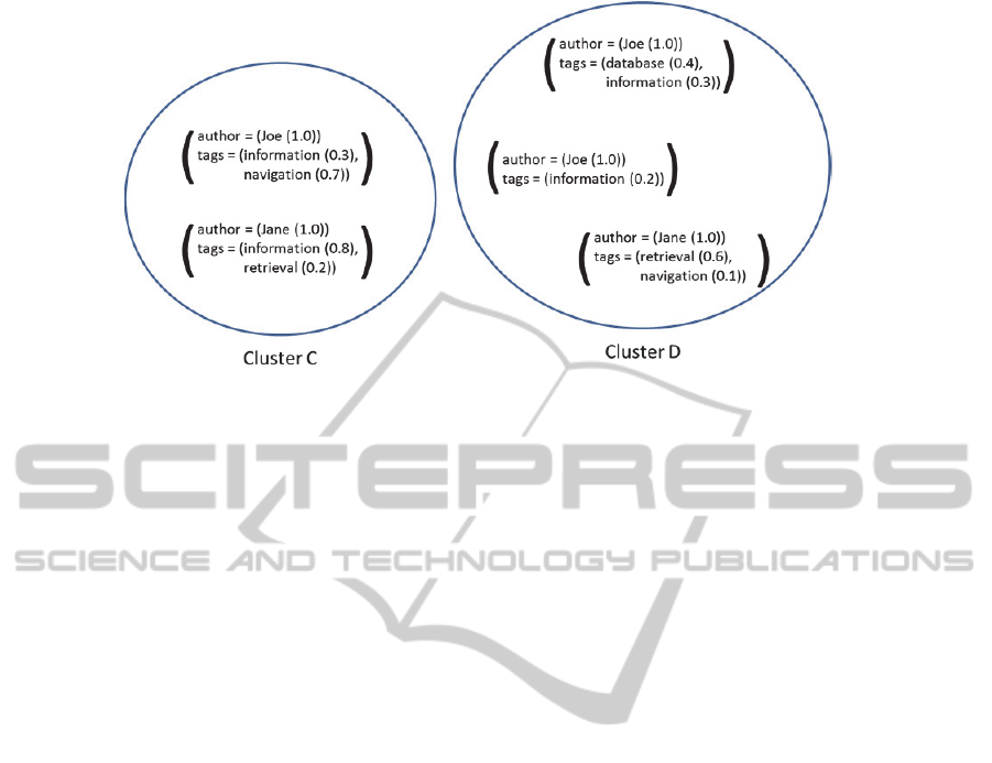
Figure 1: Two clusters with resource representations.
Our approach to learning a multi-branched topic
tree is based on the insight that HAC merge
operations happen for a certain reason, namely
because two clusters share certain characteristics. If
a dendogram node v is created out of several
consecutive cluster merges that happened for the
same (or a very similar) reason we can collapse all
the involved nodes into their parent node v because
they all share the same characteristics.
Hence, we first need to provide a concise
definition of the “reason” why two clusters are
merged or, more generally, why they are similar. We
call this notion similarity explanation.
5.1 Resource Representation
We first choose a way of representing resources –
our aim is to formulate it as generically as possible
such that it will work for all kinds of resources and
collections.
We assume that resources in an information
system can be described through a set of attributes
,…,
, each of which is defined over a set of
elements that form the basis of a vector space
.
This assumption presumes that all string
attributes can be broken into sub-structures that will
form the basis of a vector space – in most cases
these structures will be words, but for shorter string
attributes, they could also be characters or character
n-grams.
A resource is described by a list of vectors
,…,
, where vector
describes the resource in terms of attribute
and
where the jth entry of that vector, denoted
,
expresses the importance of the jth element for that
resource. In the case of a content attribute, the
weights
can be computed e.g. as the tf.idf of
term j.
As an example, consider the five resource
representations in the two clusters depicted in Figure
1: each of them has the two attributes “author” and
“tags”. The vector space for the author attribute is
spanned by the elements “Joe” and “Jane”, the
vector space for the “tags” attribute is spanned by
“information”, “navigation”, “retrieval” and
“database”. For better readability, the figure shows
only the non-zero elements of the vectors
and , with the weights
and
in brackets behind the
corresponding element.
Other attributes are of course thinkable, e.g. title,
content, creation and/or modification dates or anchor
texts for hyperlinked collections.
5.2 A Generic Distance Measure for
Resources
The distance measure that we propose is a simple
linear convex combination of partial distances, one
for each attribute. More precisely, the distance
between two resources, described by lists of vectors
U and V is computed as
,
,
Where
are weights to be chosen freely, but
under the condition that
∑
1. The partial
distances
need to be suitable to compare vectors
for attribute
– e.g. cosine-based distance for
content.
WhereDidI(T)PutIt?-AHolisticSolutiontotheAutomaticConstructionofTopicTreesforNavigation
197
5.3 Similarity Explanations
As outlined above, we now want to introduce the
concept of similarity explanation – essentially a
summary of the characteristics shared by two
clusters.
A similarity explanation is similar to a resource
representation as outlined in section 5.1, i.e. it
consists of several explanations, one for each
attribute, and each explanation is a vector over the
same vector space as defined above – only that now
the vector weights express to what degree a certain
element is shared among the two clusters.
Formally, this can be captured as follows: for
two clusters, i.e. sets of resources
,…,
and
,…,
, the similarity explanation is
defined as:
,
,
,…,
,
where each
,
denotes the vector of shared
characteristics for attribute
,defined over the
vector space
.
The weights of these vectors are defined by
looking at all possible pairs that can be formed out
of the resources in clusters C and D and seeing how
many of these pairs share the given element (e.g. tag
or keyword):
,
|
,
∈x|
0
0|
||∙||
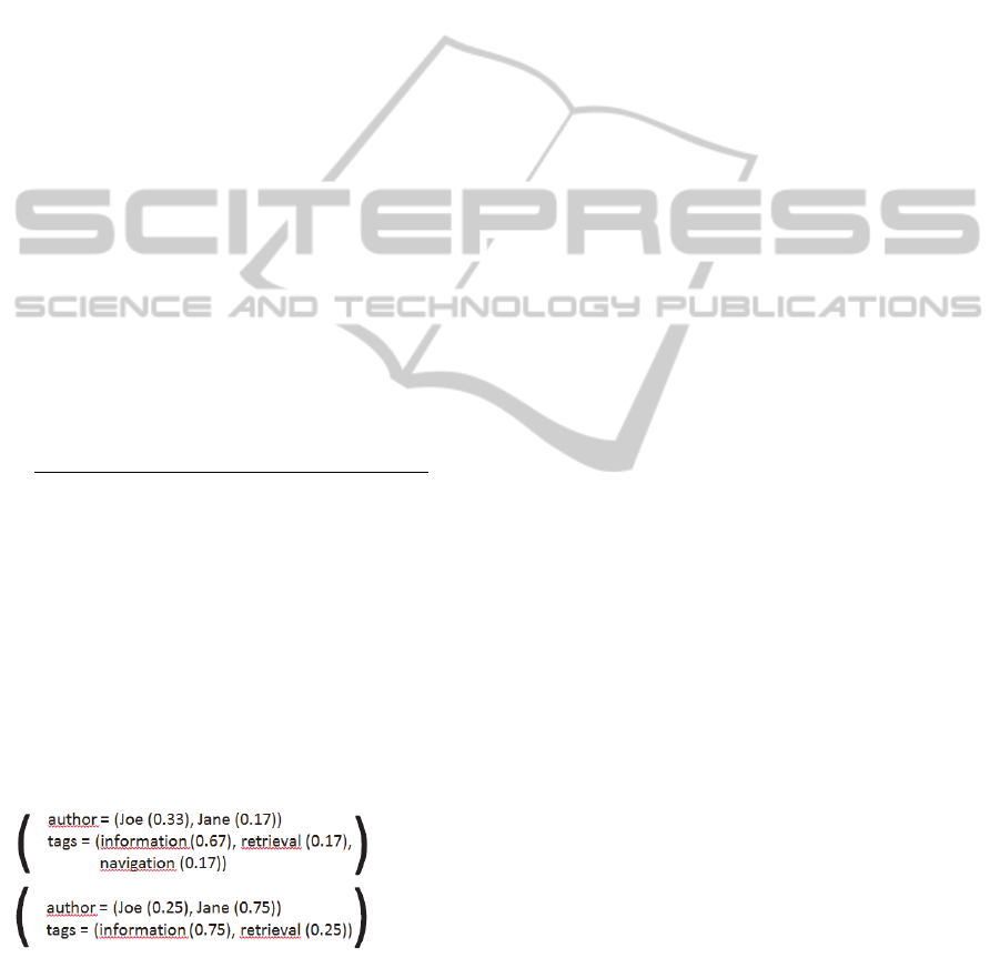
As an example, consider again the two clusters in
Figure 1: their similarity explanation is given in
Figure 2 at the top. For instance, we see that
,
0.33. This is because there is a
total of six pairs that can be formed out of the
resources in C and D (denominator) and 2 of these
pairs share the author “Joe” (numerator). Thus, we
can say that if we merged the two clusters, the
“reason” for this would be mainly that they share the
keyword “information” and that “Joe” is rather often
a shared author.
Figure 2: Similarity explanation for the two clusters from
Figure 1 (top) and another similarity explanation (bottom).
Finally, we need to capture the notion of two
cluster merges happening for “nearly the same
reason”, i.e. we need to find a way to test if two
similarity explanations are very similar. We
therefore define a measure of similarity between two
explanations as follows: let , and
,
be two similarity explanations. Then, their similarity
is defined as a weighted sum of partial similarities
for the different attributes (using the same weights
as in the distance function in section 0):
,
,,
,
,
,
The partial similarities are defined as follows:
,
,
,
1|,
,
0
0.01
Here, |,
,
| captures
in how far the two explanations differ regarding
element j. A constant smoothing factor of 0.01 is
used when that difference becomes maximal. The
rationale of using a product here is that two
explanations must show a good overlap in all
elements in order to be considered as “nearly the
same reason”.
Let us consider the two similarity explanations
given in Figure 2, and focus on the author attribute
as an example. We get
1
|
0.330.25
|
∙
1
|
0.170.75
|
0.92∙
0.42 0.39. Note that this value is fairly small
since Jane plays a much higher role in the second
explanation than in the first – we therefore regard
the two explanations as only slightly similar, i.e. the
two merges did not happen for “nearly the same
reason”.
5.4 Inferring a Multi-Branch Tree
from a Binary One
We are now ready to define our topic tree building
algorithm. It proceeds as follows:
- All the resources in the collection are clustered
with hierarchical agglomerative clustering
(HAC, (Cios et al. 1998)). The resulting
dendogram is cut at a certain level (given by a
user-defined distance threshold) – the resulting
flat clustering defines the set of dossiers (see
section 2). After that cut, the upper part of the
dendogram – with the dossiers as leaf nodes –
will be further processed. We call this tree .
- A new tree ′ – the future topic tree – is
initialized. Its new root node is mapped to the
root node of
KMIS2014-InternationalConferenceonKnowledgeManagementandInformationSharing
198

- Starting from the root node, a breadth-first
search (BFS) is performed on .
- For each inner node - with children and
and sibling node – that is processed during
BFS, the similarity explanations
,
and
,
are compared (see example in Figure
3). That is, we check whether clusters and
were merged into for the same reason as
and were merged into .
- If this is the case, i.e. if
,
,
,
for some
threshold , then is mapped to the same node
as – we call this node
.
- Otherwise, a new node
is created in
, is
mapped to ′, and
is attached as a child to
- Finally, leaf nodes of (dossiers) are mapped to
the same node as their parent.
After completion of BFS, each node in is mapped
to a node in ′ (where many nodes of can be
mapped to the same node in ′). Together with this
mapping,
constitutes the new topic tree. Note that,
with this algorithm, dossiers can be mapped to inner
nodes (even the root node) of ′.
Figure 3: Example comparison in dendogram search.
5.5 Cluster Labeling
To support proper navigation, topic tree nodes need
meaningful labels. As outlined in section 4, the label
of a parent node should express what characteristics
are shared by all its children and the labels of the
children should express individual characteristics,
but should not repeat characteristics already used to
describe the parent (assuming that users navigate a
tree top-down).
Our hypothesis is that such labels can be derived
from our similarity explanations: when a set of
dendogram nodes is mapped to a topic tree node
, then this is because these nodes were created
for the same reason during clustering. This “reason”
(i.e. similarity explanation) must be different from
the reasons for which the child nodes of
were
created in
– otherwise the child nodes would have
been mapped to ′, too. However, this does not
mean that the similarity explanation vectors of a
parent node are orthogonal to those of its children –
usually, child nodes “inherit” the characteristics of
the parent node’s similarity explanation, and exhibit
some additional characteristics that differentiate
from the parent.
We hence propose the following labeling
algorithm:
- For each node w
ϵT
, fetch the first node
such that is mapped to
.Let and
be the children of in .
- Generate a preliminary label for
that consists
of all the elements with non-zero weights in
,
.For instance the label of the node to
which node w in Figure 3 is mapped, will be
“Joe, Jane, information, retrieval”
- Iterate again over all nodes w
ϵT
and remove
all elements from the label of ′ which are
already contained in the label of its parent node.
The last step of this procedure ensures that
descriptions of child nodes do not repeat
characteristics already present in their parent nodes.
In order to evaluate the quality of labels
generated from similarity explanations (henceforth
called SE labels), we implemented a second labeling
method for comparison. That method is a special
case of the labeling method proposed in
(Treeratpituk & Callan 2006). There, a so-called
DScore is assigned to each candidate keyphrase. The
DScore is a linear combination of 11 factors,
combined using weights
. In our implementation,
we used
0, except for
and
. This means
that a keyphrase receives a high score if it appears in
many resources of the cluster to be labeled and if it
is ranked higher in the top terms of that cluster
(where top terms are again ranked by number of
cluster resources containing them) than in the top
terms of the parent cluster.
6 EVALUATION
6.1 Experimental Setup
For our evaluation, we used a test collection from
our application scenario, as described in section 2,
comprising 1474 documents. A manually created
topic tree exists for this collection and was used in
the experiment.
Resources in this collection have the attributes
title, author, tags and (often) unstructured textual
WhereDidI(T)PutIt?-AHolisticSolutiontotheAutomaticConstructionofTopicTreesforNavigation
199
content. Each of these fields can be empty for a
resource. We prepared the experiment as follows:
- Each resource in the collection was represented
using sets of vectors for all attributes, as
described in section 5.1. For distance
computations, weights were set to 0.3 (title), 0.2
(content) and 0.5 (tags) based on preliminary
experiments.
- A topic tree was built following the algorithm in
section 5.4. The parameter was set to 0.6.
- The nodes of the resulting tree were labeled,
firstly with the method based on similarity
explanations (SE-labels) and, secondly with our
variant of DScore (DScore-labels), see section
5.5. For DScore, we set
0.6 and
0.4.
- All three trees – i.e. the manually created one,
the one with SE-labels and the one with
DScore-labels – were transformed into a
hierarchy of folders on a file system, where the
inner nodes of the topic tree became folders and
the label of those nodes became the folder
names. For each resource a text file was created,
with the resource title as file name.
- 10 resources were chosen completely at random
from the entire collection. Then, 4 of these were
selected manually, such that a mixture of
different resource types (with and without
textual content) was achieved and such that it
was possible to guess roughly from the title,
content and tags what the resource was about.
- For each of the 4 chosen resources (henceforth
called test cases), a description was generated,
consisting of the title, author, tags and the most
important keywords from the content.
Then, two test persons from our institute – who
had no knowledge of the resource collection – were
chosen. This simulates a new employee joining a
company and starting to get familiar with the
collection of resources of that company.
Each test person was given the task to locate the
four test cases within each of the three topic trees,
based on the description of each test case.
Test person 1 started with the automatically
created trees whereas test person 2 first looked at the
manually created one. This was done to exclude a
bias due to test persons learning about test cases
while searching.
We then recorded the search process with a
screen capturing software and measured the time
needed to locate each test case, as well as the
number of “backtracks” during search. Afterwards,
the test persons were asked about their impressions
of the search process with the different topic trees.
(a)
(b)
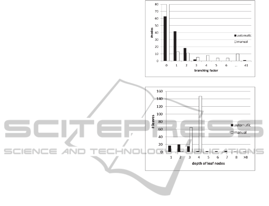
Figure 4: Histogram of (a) branching factor and (b) depth
of leaf nodes for both trees.
6.2 Results
First, we want to characterize the nature of the topic
trees. Figure 4 (a) shows a histogram of the
branching factors of all nodes in both trees. We can
see that most nodes in the automatic tree have
between 0 and 2 children. Only the root node has 41
children. Most nodes in the manually created tree are
leaves (214, not visible due to cut y-axis) and most
inner nodes have between 1 and 6 children (the root
node has 5 children).
Figure 4 (b) shows a histogram of the depths of
leaf nodes. Here, we can see that 83% of all leaves
in the automatic tree reside at a depth between 1
(directly beneath the root) and 3. In the manual tree,
virtually all leaves reside at a depth of either 3 or 4.
This means that the manually created tree is also
quite flat, but much better balanced at all levels.
Table
1
shows the time that the test persons
needed to locate each test case in each of the trees.
Cases where the search was given up are marked
with asterisks (*). In addition, the table lists the
number of backtracks (i.e. number of times a dead-
end was reached and upward navigation occurred),
divided by the length of the search in minutes.
KMIS2014-InternationalConferenceonKnowledgeManagementandInformationSharing
200

The first observation is that in 7 out of 8 test
instances (4 test cases times two persons), the SE-
labeled tree led to a faster result than the manual
tree. This is rather strong evidence that – for the
given search scenario – an automatically constructed
and properly labeled tree can lead to more efficient
search and browsing than a manually created tree.
The comparison between SE-labels and DScore
is more inconclusive: SE-labels are more efficient in
only 5 out of 8 cases.
Table 1: Summary of time needed to locate test cases, and
number of backtracks per minute. Cases that were given
up are marked with *.
Test
Case
Tree Testperson 1 Testperson 2
Time
(sec.)
Back-
tracks/
min.
Time
(sec.)
Back-
tracks/
min.
1
Manual 595* 2.9 270* 2.7
SE-labels 202 1.8 173 0.3
DScore
32
0
58
1.0
2
Manual 65 0.9 191 3.8
SE-labels
45
0
20
0
DScore 191 1.3 38 0
3
Manual 96 3.8 310* 7.5
SE-labels
21
0
58
1.0
DScore 73 0.8 87 0
4
Manual 329 2.4 131 0.9
SE-labels
226
1.1 456* 1.4
DScore 590* 1.5
115
1.0
The analysis of backtracking frequency clearly
shows that in the manual tree much time is spent on
exploring dead ends (backtrack rate being above
2.4/min. in 6 out of 8 cases), whereas – as expected
– the automatically created trees require much time
for looking at the (many) top-level nodes, but have
much fewer backtracks (well below 2/min. in all
cases, often even 0).
We finally summarise the verbal feedback of our
two test persons: both of them stated that they were
surprised how well they were able to work with the,
at first glance, seemingly cryptical automatic tree.
It also became clear – and was remarked by one
test person – that our evaluation scenario is only
valid under the assumption of a new employee
getting familiar with a topic tree. It was apparent
that the manually constructed tree required more
background knowledge about the way of organizing
things in our example company (including e.g. the
meaning of abbreviations) – something that an
experienced employee might exploit for very fast
navigation in the manual tree. For a more general
evaluation, it would hence be necessary to elicit real
information needs and repeat the search experiment
with these. The inconclusiveness of the comparison
of the two automatic labeling methods was
confirmed by the verbal feedback: one test person
preferred the SE-labels, the other the DScore labels.
7 CONCLUSIONS AND FUTURE
WORK
We could show that replacing or complementing
manually created navigation structures by
automatically created ones can significantly fasten
retrieval and that automatic clustering can help to
decrease the danger of missing relevant information
because all versions of the same document are
clustered into the same nodes.
Our work is based on existing approaches for
clustering and labeling but focuses on yet
unrewarding aspects. Evaluation was done by
involving test persons and based on a comparison of
retrieval time for finding given documents in
manually and automatic generated information
structures and proved the advantage of automatically
created topic trees (either with SE-labels or DScore-
labels).
Further research will detail and refine our
approach and also investigate alternative methods,
e.g. divisive instead of agglomerative clustering and
re-evaluation on a broader scale.
Starting point for the next evaluation circle will
then be a real information need, e.g. a request for
finding a specific offer triggered by the call of a
customer. Evaluators will be persons familiar with
the organizational context of the search.
REFERENCES
Alfred, R. et al., 2014. Concepts Labeling of Document
Clusters Using a Hierarchical Agglomerative
Clustering (HAC) Technique. In The 8th International
Conference on Knowledge Management in
Organizations. pp. 263–272.
Blundell, C., Teh, Y. W. & Heller, K., 2010. Bayesian
Rose Trees. In Proceedings of UAI-10. pp. 65–72.
Bruls, M., Huizing, K. & Van Wijk, J.J., 2000. Squarified
treemaps. In Data Visualization 2000. Vienna,
Austria: Springer, pp. 33–42.
Caraballo, S., 1999. Automatic Acquisition of a
hypernym-labeled noun hierarchy from text. In
Proceedings of the Association for Computational
Linguistics Conference.
Chuang, S.-L. & Chien, L.-F., 2004. A practical web-
based approach to generating topic hierarchy for text
segments. In Proceedings of CIKM ’04. p. 127.
WhereDidI(T)PutIt?-AHolisticSolutiontotheAutomaticConstructionofTopicTreesforNavigation
201

Cios, K., Pedrycz, W. & Swiniarski, R. W., 1998. Data
mining methods for knowledge discovery, Norwell,
MA, USA: Kluwer Academic Publishers.
Cutting, D. R., Karger, D. R. & Pedersen, J.O., 1993.
Constant interaction-time scatter/gather browsing of
very large document collections. In Proceedings of
SIGIR ’93. pp. 126–134.
Glover, E. et al., 2002. Inferring hierarchical descriptions.
In Proceedings of CIKM ’02. ACM Press.
Lawrie, D., Croft, W. B. & Rosenberg, A., 2001. Finding
topic words for hierarchical summarization. In
Proceedings of SIGIR ’01. ACM Press, pp. 349–357.
Lutz, J., Thönssen, B. & Witschel, H.F., 2013. Breaking
free from your information prison. A recommender
based on semantically enriched context descriptions.
In 1st International Conference on Enterprise Systems.
Muller, A. et al., 1999. The TaxGen framework:
automating the generation of a taxonomy for a large
document collection. In Proc. of HICSS-32. p. 9.
Popescul, A. & Ungar, L. H., 2000. Automatic labeling of
document clusters. Available at: http://citeseer.nj.
nec.com/popescul00automatic.html.
Radev, D.R. et al., 2004. Centroid-based summarization of
multiple documents. Information Processing &
Management, 40(6), pp.919–938.
Thönssen, B., 2013. Automatic, Format-independent
Generation of Metadata for Documents Based on
Semantically Enriched Context Information.
University of Camerino.
Treeratpituk, P. & Callan, J., 2006. Automatically labeling
hierarchical clusters. In Proceedings of dg.o ’06.
ACM Press, p. 167.
Zavitsanos, E., Paliouras, G. & Vouros, G. A., 2011. Non-
Parametric Estimation of Topic Hierarchies from
Texts with Hierarchical Dirichlet Processes. The
Journal of Machine Learning Research, 12, pp.2749–
2775.
KMIS2014-InternationalConferenceonKnowledgeManagementandInformationSharing
202
