Singularity Stairs Following with Limited Numbers of Hidden Units
Seiya Satoh and Ryohei Nakano
Department of Computer Science, Chubu University, 1200 Matsumoto-cho, Kasugai 487-8501, Japan
Keywords:
Multilayer Perceptron, Learning Method, Singular Region, Reducibility Mapping.
Abstract:
In a search space of a multilayer perceptron having J hidden units, MLP(J), there exist flat areas called singular
regions that cause serious stagnation of learning. Recently a method called SSF1.3 utilizing singular regions
has been proposed to systematically and stably find excellent solutions. SSF1.3 starts search from a search
space of MLP(1), increasing J one by one. This paper proposes SSF2 that performs MLP search by utilizing
singular regions with J changed bidirectionally within a certain range. The proposed method was evaluated
using artificial and real data sets.
1 INTRODUCTION
In a multilayer perceptron (MLP) search space, there
exist flat areas called singular regions where gradients
are zero and the corresponding input-output maps are
the same (I-O equivalent) (Sussmann, 1992). Since
most learning methods get stuck in singular regions,
a method (Amari, 1998) was once proposed so as to
avoid singular regions, but there is no guarantee that
avoiding singular regions will provide an excellent so-
lution.
Statistical models having singular regions are
called singular models, and many useful models such
as MLPs, RBFs, Gaussian mixtures, and HMMs are
singular models (Watanabe, 2009). Learning the-
ory of singular models has been studied intensively
(Watanabe, 2008; Watanabe, 2009); however, empir-
ical studies of singular models have been scarcely
done. As partial knowledge, we know that an MLP
search space has extensive flat areas and troughs
(Hecht-Nielsen, 1990), or most points along a search
route have huge condition numbers (Nakano et al.,
2011). Moreover, an MLP search space has many
equivalent points due to equivalence relations (Suss-
mann, 1992) caused by permutations of hidden units
or the nature of an activation function. Even after ex-
cluding such equivalences, an MLP search space may
have local optima (Duda et al., 2001).
A completely new learning method SSF (Singu-
larity Stairs Following) (Nakano et al., 2011) making
good use of singular regions was proposed to stably
and successively find excellent solutions of an MLP.
SSF1.2 (Satoh and Nakano, 2013) extended the orig-
inal so as to cover all kinds of singular regions and to
reduce the number of starting points. SSF1.3 (Satoh
and Nakano, 2014) accelerates SSF1.2 by introducing
search pruning without deteriorating solution quality.
This paper proposes a new method called SSF2
which performs MLP search by making good use of
singular regions with the number of hidden units J
changed bidirectionally within a certain range. The
method was evaluated using artificial and real data.
2 SINGULAR REGIONS OF
MULTILAYER PERCEPTRON
2.1 Reducibility Mapping and Singular
Regions
Let MLP(J) be an MLP having J hidden units. This
section explains howwe can generate singular regions
in MLP(J) search space by applying reducibility map-
pings to the optimum of MLP(J−1) (Fukumizu and
Amari, 2000).
We consider MLP(J) having one output unit. The
output for input x is defined as below. Here parame-
ters θ
J
= {w
0
,w
j
,w
j
, j = 1,··· ,J} and g(h) is an acti-
vation function, where w
j
is a vector of weights from
all input units to hidden unit j, and w
j
is a weight
from hidden unit j to the single output.
f
J
(x;θ
J
) = w
0
+
J
∑
j=1
w
j
z
j
, z
j
≡ g(w
T
j
x) (1)
180
Satoh S. and Nakano R..
Singularity Stairs Following with Limited Numbers of Hidden Units.
DOI: 10.5220/0005075601800186
In Proceedings of the International Conference on Neural Computation Theory and Applications (NCTA-2014), pages 180-186
ISBN: 978-989-758-054-3
Copyright
c
 2014 SCITEPRESS (Science and Technology Publications, Lda.)

Given data {(x
µ
,y
µ
),µ = 1,··· ,N}, we try to find
MLP(J) which minimizes the following:
E
J
≡ E(θ
J
) =
1
2
N
∑
µ=1
( f
µ
J
− y
µ
)
2
, (2)
f
µ
J
≡ f
J
(x
µ
;θ
J
).
We also consider MLP(J−1) having parameters
θ
J−1
= {u
0
,u
j
,u
j
, j = 2, · · · ,J}. The output is defined
as below.
f
J−1
(x;θ
J−1
)=u
0
+
J
∑
j=2
u
j
v
j
, v
j
≡g(u
T
j
x) (3)
Now we consider the following three reducibility
mappings α, β, and γ. Let
b
Θ
α
J
,
b
Θ
β
J
, and
b
Θ
γ
J
be the
regions obtained by applying mappings α, β, and γ
respectively to the optimum
b
θ
J−1
.
b
θ
J−1
α
−→
b
Θ
α
J
,
b
θ
J−1
β
−→
b
Θ
β
J
,
b
θ
J−1
γ
−→
b
Θ
γ
J
b
Θ
α
J
≡ {θ
J
| w
0
= bu
0
, w
1
=0, (4)
w
j
= bu
j
,w
j
=bu
j
, j=2,··· , J}
b
Θ
β
J
≡ {θ
J
| w
0
+w
1
g(w
10
)= bu
0
, (5)
w
1
=[w
10
,0,··· ,0]
T
,
w
j
= bu
j
,w
j
= bu
j
, j=2,··· ,J}
b
Θ
γ
J
≡ {θ
J
| w
0
= bu
0
, w
1
+ w
m
= bu
m
, (6)
w
1
=w
m
=bu
m
,
w
j
= bu
j
,w
j
=bu
j
, j∈{2,··· , J}\{m}}
From the above, the following two kinds of singular
regions are formed in MLP(J) search space. One is
b
Θ
αβ
J
, the intersection of
b
Θ
α
J
and
b
Θ
β
J
. The parameters
are as follows, and only w
10
is free.
w
0
= bu
0
, w
1
= 0, w
1
= [w
10
,0,··· ,0]
T
w
j
= bu
j
, w
j
= bu
j
, j = 2, · · · ,J (7)
The other is
b
Θ
γ
J
, having the following restriction.
w
1
+ w
m
= bu
m
(8)
2.2 SSF1.3 (Singularity Stairs Following
ver. 1.3)
The search method SSF1.3 (Satoh and Nakano, 2014)
finds solutions of MLP(J) successively from J=1 un-
til J
max
making good use of singular regions of each
MLP(J). Since gradients are zero at points in a sin-
gular region, we employ eigenvector descent (Satoh
and Nakano, 2012) only at a starting point, and em-
ploy BPQ (BP based on Quasi-Newton) (Saito and
Nakano, 1997), a kind of quasi-Newton,from then on.
Eigenvector descent calculates the Hessian matrix H,
and then as a search direction pick up the eigenvector
corresponding to each negative eigenvalue of H.
SSF1.3 has the following characteristics.
(1) Since most points in singular regions are saddles
(Fukumizu and Amari, 2000), SSF1.3 can descend to-
ward a better solution, thus guaranteeing monotonic
decrease of training error.
(2) SSF1.3 does not have to be repeated since random
numbers are not used in SSF1.3.
(3) SSF1.3 finds a set of solutions for successive J =
1,··· ,J
max
, which can be quite useful for model se-
lection.
(4) During each search process, the possibility of
search pruning is checked if the current search will
merge into any existing search route. If a positive re-
sult is obtained, the search is pruned.
3 PROPOSED METHOD: SSF2
As stated above, SSF1.3 finds excellent solutions suc-
cessively for J = 1,··· , J
max
. However, when we are
interested in a large J and solutions for a smaller J
are not necessary, we can omit search for a smaller
J. This paper proposes a new version of SSF called
SSF2, which performs MLP search by utilizing sin-
gular regions with J changed bidirectionally within a
certain range. How to change J bidirectionally is not
defined here, which is to be investigated.
3.1 General Flow of SSF2
The procedure of SSF2 is described below. Here
[J
min
,J
max
] is a range of J to examine, and up is a flag
where up = 1 means J is in an increase phase and up
= 0 means a decrease phase.
SSF2 (Singularity Stairs Following 2):
1. Set values for J, J
min
, J
max
and up.
2. Find solutions of MLP(J) from random starting
points, and keep the best as the optimum of
MLP(J),
b
θ
J
.
3. Repeat the following:
3.1. if up = 1 then do (a), otherwise do (b).
(a) Apply reducibility mapping to
b
θ
J
to get sin-
gular regions, and find solutions of MLP(J+1)
by starting from the regions. Store the best as
the optimum
b
θ
J+1
.
J ← J + 1. if J=J
max
, then up ← 0.
(b) Find solutions of MLP(J−1) by starting
SingularityStairsFollowingwithLimitedNumbersofHiddenUnits
181

from
b
θ
J
and using the decrement method de-
scribed in the next section, and store the best as
the optimum
b
θ
J−1
.
J ← J − 1. if J=J
min
, then up ← 1.
3.2. if one of stopping criteria is satisfied, then
stop.
3.2 Decrement Method
Decrement method decreases the number of hidden
units, which is required in step 3.1 (b) stated above.
Given
b
θ
J
, the optimum of MLP(J), we want to find
b
θ
J−1
, the optimum of MLP(J−1).
One may consider just deleting one of the hidden
units from
b
θ
J
and then starting search. However, such
simple deletion is too naive to obtain an excellent so-
lution, as shown in our experiments. Here we con-
sider a method which guides search of MLP(J) from
b
θ
J
into a singular region, and then deletes the redun-
dant hidden unit. Note that we have two kinds of sin-
gular regions.
First, we consider guiding search into singular re-
gion
b
Θ
αβ
J
. Let m be the hidden unit to delete. Perform
learning of MLP(J) with w
m
and w
m
fixed as follows.
w
m
← a× bw
m
, w
m
← a × bw
m
(9)
Here a is changed gradually from 1 to 0, guiding
search into
b
Θ
αβ
J
. After finishing search with a=0, we
delete hidden unit m to get
b
θ
J−1
. As for m, we can se-
lect a small number of candidates in ascending order
of |w
m
| or try all cases.
Next, we consider guiding search into singular re-
gion
b
Θ
γ
J
. Let m and n be the hidden units to merge.
Perform learning of MLP(J) with w
m
and w
n
fixed as
follows.
w
m
← b× bw
m
+ (1− b) × bw
n
, (10)
w
n
← b× bw
n
+ (1− b) × bw
m
(11)
Here b is changed from 1 to 0.5, guiding search into
b
Θ
γ
J
. After finishing search of MLP(J) with b=0.5, up-
date w
m
as w
m
← w
m
+ w
n
, delete hidden unit n, and
then perform learning of MLP(J−1) to get
b
θ
J−1
. As
for m and n, there are J × (J − 1)/2 combinations;
thus, trying all cases would be unrealistic. We can
select a small number of pairs in ascending order of
distance kw
m
− w
n
k.
4 EXPERIMENTS
We evaluated the proposed SSF2 for the following
sigmoidal MLP using artificial and real data. Here
σ(h) = 1/(1+ exp(−h)).
f = w
0
+
J
∑
j=1
w
j
z
j
, z
j
= σ(w
T
j
x) (12)
For comparison, we used a quasi-Newton called BPQ
and SSF1.3. The initial weights for BPQ are ran-
domly selected from the range [−1, +1] with the ex-
ception w
0
=
y. BPQ was repeated 100 times for each
J.
For SSF1.3 and the increase phase of SSF2, we
set free parameters of the singular regions as follows.
For
b
Θ
αβ
J
we set as w
10
=0 and for
b
Θ
γ
J
we set q in the
following as q=0.5, 1.0, and 1.5.
w
1
← q× bu
m
, w
m
← (1− q) × bu
m
(13)
For SSF1.3 and SSF2, search pruning check was done
for each 100 points during search.
We started SSF2 with J=J
max
and up=0. The best
solution obtained by running BPQ 20 times was se-
lected as the optimum
b
θ
J
at the initial J (=J
max
). In
our experiments, SSF2 went in one cycle with J de-
creased from J
max
to J
min
, then increased from J
min
to
J
max
, and stopped.
Each search was stopped when the iteration ex-
ceeded 10,000 sweeps, or the search step got smaller
than 10
−16
. Test error for artificial data was calculated
15 20
10
0
10
1
training error
J
BPQ
SSF1.3
SSF2(1 step)
SSF2(3 steps)
SSF2(10 steps)
(a) training error
5 10 15 20
1e−1
1e0
1e1
1e2
1e3
1e4
1e5
1e6
1e7
test error
J
(b) test error
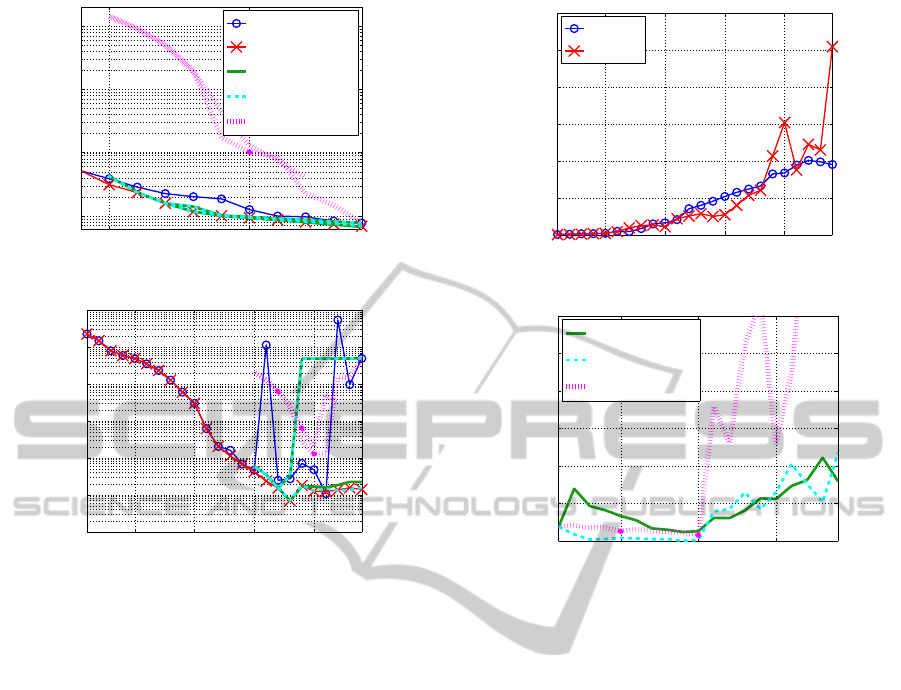
Figure 1: Solution quality for Experiment 1a.
NCTA2014-InternationalConferenceonNeuralComputationTheoryandApplications
182

using test data of 1,000 data points without noise,
generated independently of training data. Test error
for real data was evaluated using one segment among
10 segments; the remaining 9 segments were used for
training.
4.1 Experiment using Artificial Data
Our artificial data set was generated using MLP hav-
ing weights shown in the following equations. Values
of variables x
1
,··· , x
10
were randomly selected from
the range (0,1). Note that five variables x
1
,··· ,x
5
contribute to y, but the other five variables x
6
,··· ,x
10
are irrelevant. We included irrelevant variables to
make the learning harder. Values of y were generated
by adding small Gaussian noise N (0,0.05
2
) to MLP
outputs. The sample size was 1,000 (N=1,000). We
set J
min
=15 and J
max
=24, while the original J=22.
[w
0
,w
1
,··· ,w
22
]
= [−11,−12,−10,−6,4,20,18,−3, 12,−18,−17,17,−1,
13,−9,9,−3,14,1− 18,15,12, 13],
[w
1
,w
2
,··· ,w
22
]
=







3 −7 −2 6 −8 7 −3 10 −5 10 −3
−3 3 −6 2 −7 −8 9 2 3 1 −5
9 1 4 −1 −4 −3 −8 2 −4 1 −9
−8 −8 3 −6 −7 −10 1 5 0 2 −4
3 −4 5 7 −9 −4 −4 0 4 6 −8
−10 −6 −1 2 4 5 −10 −9 −5 −3 2
−1 1 10 −6 −7 1 −1 3 −3 7 −6
0 0 −8 2 −7 −4 3 −3 −7 3 10
−5 −10 −8 9 −7 −9 −2 −2 1 4 −1
5 8 6 −1 9 −6 3 −1 5 −2 0
6 2 −2 2 10 4 −10 8 −9 −5 3
2 −2 −5 9 −8 5 4 −3 7 6 5







In our experiments using artificial data, we
examine how the performance of SSF2 is influenced
by our decrement method. Below we examined in
two ways 1a and 1b.
(1) Experiment 1a
First, in the decrement method, only singular re-
gion
b
Θ
αβ
J
was considered, and every hidden unit
was tested as a candidate to delete. In eq. (9), we
changed the number of guiding steps in three ways:
one step, three steps (a = 2/3, 1/3,0), and ten steps
(a = 9/10,8/10, · · · ,1/10,0). They are referred to as
SSF2(1 step), SSF2(3 steps), and SSF2(10 steps) re-
spectively. Note that SSF2(1 step) is nothing but sim-
ple deletion.
Figure 1 shows the solution quality of each
method, showing the best training errors and cor-
responding test errors. Each SSF2 method made a
round trip, at first decreasing J from 24 until 15, and
then increasing J until 24, while SSF1.3 went on in-
creasing J. SSF1.3 outperformed BPQ both in train-
ing and test. In each SSF2 method, the second half
5 10 15 20
0
1000
2000
3000
4000
5000
6000
CPU time (sec.)
J
BPQ
SSF1.3
(a) BPQ, SSF1.3
5 10 15
0
1000
2000
3000
4000
5000
6000
CPU time (sec.)
t
SSF2(1 step)
SSF2(3 steps)
SSF2(10 steps)
(b) SSF2
Figure 2: CPU time for Experiment 1a.
(increase phase) worked better than the first half (de-
crease phase) in both training and test. SSF2(1 step)
worked rather poorly especially in test. However,
SSF2(3 steps) and SSF2(10 steps) worked in much the
same manner, and their increase phases were almost
equivalent to that of SSF1.3. SSF2(3 steps), SSF2(10
steps) and SSF1.3 indicate J=18 is the best model,
while BPQ indicates J=21 is the best.
Figure 2 shows CPU time required by each
method. The horizontal axis t in Fig. 2(b) indi-
cates how many times J was changed; thus, t=1,···,10
corresponds to the decrease phase from J=24 until
15, and t=10,···,19 means the increase phase from
J=15 until 24. Each method has a tendency to re-
quire longer CPU time as J increases. Among SSF2
methods, SSF2(1 step) spent the longest because it
required the largest number of search routes in its in-
crease phase. The total CPU time of BPQ, SSF1.3,
SSF2(1 step), SSF2(3 steps), and SSF2(10 steps)
were 5h28m, 6h30m, 7h20m, 5h1m, and 6h1m re-
spectively. Hence, both SSF2(3 steps) and SSF2(10
steps) were faster than SSF1.3.
Based on the results of Experiment 1a, we consid-
ered SSF(3 steps) as the most promising when using
only singular region
b
Θ
αβ
J
.
SingularityStairsFollowingwithLimitedNumbersofHiddenUnits
183

15 20
10
0
10
1
10
2
10
3
training error
J
BPQ
SSF1.3
SSF2(all α β)
SSF2(5 α β)
SSF2(5 γ)
(a) training error
5 10 15 20
1e−1
1e0
1e1
1e2
1e3
1e4
1e5
test error
J
(b) test error
Figure 3: Solution quality for Experiment 1b.
(2) Experiment 1b
Next, we examined two possibilities: i) as for singu-
lar region
b
Θ
αβ
J
, what if we use only top five hidden
units instead of using all, and ii) what if we use only
top five for singular region
b
Θ
γ
J
instead of using
b
Θ
αβ
J
.
They are referred to as SSF2(5 αβ) and SSF2(5 γ) re-
spectively, and will be compared with SSF2(all αβ)
which is equivalent to SSF2(3 steps) in Experiment
1a.
Figure 3 shows the best training and test errors for
each method. Each SSF2 method has two lines, indi-
cating decrease and increase phases. The training and
test errors of SSF2(5 γ) were rather large and quite
unsatisfactory. Since it required huge CPU time, the
processing was stopped at J=22 in the increase phase.
The best training and test errors of SSF2(5 αβ) were
much the same as SSF2(all αβ)=SSF2(3 steps) and
also much the same as SSF1.3.
Figure 4 compares CPU time required by each
method. The horizontal axis t in Fig. 4(b) indicates
the same meaning as in Fig. 2. SSF2(5 γ) needed
huge CPU time. The total CPU time of SSF2(all αβ),
SSF2(5 αβ), and SSF2(5 γ) were 5h1m, 4h45m, and
10h9m respectively. Note that 4h45m of SSF2(5 αβ)
was much shorter than 6h30m of SSF1.3.
Experiments 1a and 1b showed SSF2(5 αβ) was
5 10 15 20
0
1000
2000
3000
4000
5000
6000
CPU time (sec.)
J
BPQ
SSF1.3
(a) BPQ, SSF1.3
5 10 15
0
1000
2000
3000
4000
5000
6000
CPU time (sec.)
t
SSF2(all α β)
SSF2(5 α β)
SSF2(5 γ)
(b) SSF2
Figure 4: CPU time for Experiment 1b.
the best among SSF2 methods we examined. Com-
pared with SSF1.3, SSF2(5 αβ) showed much the
same solution quality and was faster.
4.2 Experiment using Real Data
We evaluated SSF2 using Parkinson telemonitoring
data (Little el al., 2007) available from UCI ML
Repository. The number of variables is 18 (K=18)
and the sample size is 5,875 (N=5,875). As for SSF2,
we used SSF2(5 αβ), which performed the best in Ex-
periment 1. Note that SSF2(5 αβ) employs only
b
Θ
αβ
J
,
only top five hidden units to delete, and three steps
guiding into the singular region. We set J
min
=13 and
J
max
=22.
Figure 5 shows the training and test errors for each
method. Here again, SSF2(5 αβ) has two lines as in
Fig. 3. From Fig. 5(a), we can see the best training
errors of SSF2 considerably outperformed the other
two. The training errors of SSF2 and SSF1.3 show
preferable monotonic decrease, while those of BPQ
showed up-and-down movement. From Fig. 5(b), we
see that the best test errors of SSF2 also outperformed
the other two.
Figure 6 shows CPU time required by each
NCTA2014-InternationalConferenceonNeuralComputationTheoryandApplications
184

5 10 15 20
10
2
10
3
training error
J
BPQ
SSF1.3
SSF2(5 α β)
(a) training error
5 10 15 20
10
2
test error
J
BPQ
SSF1.3
SSF2(5 α β)
(b) test error
Figure 5: Solution quality for Experiment 2.
method. The increase phase (t ≥ 10) of SSF2
needed very long CPU time. The total CPU time of
BPQ, SSF1.3, and SSF2 were 24h49m, 60h53m, and
105h16m respectively.
In this experiment, the solution quality of SSF2
was better than BPQ and SSF1.3, but SSF2 required
more CPU time than the other two.
5 CONCLUSION
This paper proposed SSF2 which performs MLP
search by making good use of singular regions with
J changed bidirectionally within a certain range. The
method was tuned and evaluated using artificial and
real data. Our experiments using artificial data
showed the tuned SSF2 showed much the same solu-
tion quality as the existing SSF1.3 with much smaller
CPU time. In our experimentusing real data, SSF2 re-
sulted in better solutions with longer CPU time. In the
future we will make the method even faster and exam-
ine how the range of J influences the performance.
5 10 15 20
0
1
2
3
4
5
6
x 10
4
CPU time (sec.)
J
BPQ
SSF1.3
(a) BPQ, SSF1.3
5 10 15
0
1
2
3
4
5
6
x 10
4
CPU time
t
SSF2(5 α β)
(b) SSF2(5 αβ)
Figure 6: CPU time for Experiment 2.
ACKNOWLEDGEMENTS
This work was supported by Grants-in-Aid for Sci-
entific Research (C) 25330294 and Chubu University
Grant 26IS19A.
REFERENCES
Amari, S. (1998). Natural gradient works efficiently in
learning. Neural Computation, 10 (2):251–276.
Duda, R.O., Hart, P.E. and Stork, D.G. (2001). Pattern clas-
sification. John Wiley & Sons, Inc., New York, 2nd
edition.
Fukumizu, K. and Amari, S. (2000). Local minima and
plateaus in hierarchical structure of multilayer percep-
trons. Neural Networks, 13 (3):317–327.
Hecht-Nielsen, R. (1990). Neurocomputing. Addison-
Wesley Publishing Company, Reading, Mas-
sachusetts.
Little, M.A., McSharry, P.E., Roberts, S.J., Costello D.A.E.,
Moroz, I.M. (2007). Exploiting nonlinear recurrence
and fractal scaling properties for voice disorder detec-
tion. BioMedical Engineering OnLine 2007, 6:23.
SingularityStairsFollowingwithLimitedNumbersofHiddenUnits
185

Nakano, R., Satoh, E. and Ohwaki, T. (2011). Learning
method utilizing singular region of multilayer percep-
tron. Proc. 3rd Int. Conf. on Neural Comput. Theory
and Appl., pp.106–111, 2011.
Saito, K. and Nakano, R. (1997). Partial BFGS update and
efficient step-length calculation for three-layer neural
networks. Neural Compututation, 9 (1): 239–257.
Satoh, S. and Nakano, R. (2012). Eigen vector descent and
line search for multilayer perceptron. Proc. Int. Multi-
Conf. of Engineers and Comput. Scientists, vol.1,
pp.1–6.
Satoh, S. and Nakano, R. (2013). Fast and stable learn-
ing utilizing singular regions of multilayer perceptron.
Neural Processing Letters, 38 (2): 99–115.
Satoh, S. and Nakano, R. (2014). Search pruning for a
search method utilizing singular regions of multilayer
perceptrons (in Japanese). IEICE Trans. on Informa-
tion and Systems, J97-D (2):330–340.
Sussmann, H.J. (1992). Uniqueness of the weights for min-
imal feedforward nets with a given input-output map.
Neural Networks, 5 (4):589–593.
Watanabe, S. (2008). A formula of equations of states in
singular learning machines. Proc. Int. Joint Conf. on
Neural Networks, pp.2099–2106, 2008.
Watanabe, S. (2009). Algebraic geometry and statistical
learning theory. Cambridge Univ. Press, Cambridge.
NCTA2014-InternationalConferenceonNeuralComputationTheoryandApplications
186