
Learning Kernel Label Decompositions
for Ordinal Classification Problems
M. P
´
erez-Ortiz, P. A. Guti
´
errez and C. Herv
´
as-Mart
´
ınez
University of C
´
ordoba, Dept. of Computer Science and Numerical Analysis,
Rabanales Campus, Albert Einstein Building, 14071 C
´
ordoba, Spain
Keywords:
Kernel Learning, Support Vector Machines, Ordinal Classification, Kernel-target Alignment.
Abstract:
This paper deals with the idea of decomposing ordinal multiclass classification problems when working with
kernel methods. The kernel parameters are optimised for each classification subtask in order to better adjust
the kernel to the data. More flexible multi-scale Gaussian kernels are considered to increase the goodness of
fit of the kernel matrices. Instead of learning independent models for all the subtasks, the optimum convex
combination of the kernel matrices is then obtained, leading to a single model able to better discriminate
the classes in the feature space. The results of the proposed algorithm shows promising potential for the
acquisition of better suited kernels.
1 INTRODUCTION
Kernel mapping is one of the most widespread ap-
proaches to implicitly derive nonlinear classifiers.
The crucial ingredient of kernel methods is undoubt-
edly the application of the so-called kernel trick
(Vapnik, 1998), which maps the data into a higher-
dimensional feature space H via some mapping Φ.
This allows the formulation of nonlinear variants of
any algorithm that can be cast in terms of inner prod-
ucts between data points. Instead of explicitly com-
puting the function Φ, H can be efficiently obtained
from a suitable kernel function, such as the Gaussian
one. A poor choice of this function can lead to signifi-
cantly impaired performance since it implicitly deter-
mines the feature space H . Usually, a parametrised
set of kernels is chosen, although it is still necessary
to choose a performance measure and an optimisation
strategy leading to the best kernel function. This op-
timisation is often performed using a grid-search or
cross-validation procedure over a previously defined
search space. However, other strategies have been
developed, such as kernel target alignment (Cristian-
ini et al., 2002; Ramona et al., 2012; Chapelle et al.,
2002).
Among all kernel methods, support vector ma-
chines (SVM) (Cortes and Vapnik, 1995) are the most
popular ones. Given that SVMs are originally for-
mulated for binary classification, multiclass problems
are faced by decomposing them into several binary
subproblems (Hsu and Lin, 2002). Apart from the
nominal multiclass setting, there are also other learn-
ing settings for which binary decomposition are usu-
ally considered, e.g. ordinal classification, a learn-
ing paradigm covering those classification problems
where an order between the labels exist (Waegeman
and Boullart, 2009). This paper proposes a technique
for kernel learning in ordinal regression based on de-
composing the original task into several subtasks and
obtaining one single final kernel matrix. Concerning
ordinal classification, different kernel-based methods,
which were specially designed for this learning set-
ting, have emerged over the past few years, such
as several formulations of SVM (Chu and Keerthi,
2007; Shashua and Levin, 2003), the reformulation of
the standard kernel discriminant analysis (Sun et al.,
2010) or probabilistic ordinal models (P
´
erez-Ortiz
et al., 2013). Most of these approaches share the com-
mon objective of projecting the patterns to a line in
such a way that the classes are ordered according to
their ranking. Different thresholds are then derived in
order to divide the line and provide an unique ordinal
prediction. However, none of the proposed techniques
has focused on the optimisation of this kernel matrix,
which is the main objective of this paper (therefore,
our proposal can be applied to any of the aforemen-
tioned methods).
On the other hand, some works suggest the use
of kernel functions with more degrees of freedom
(Chapelle et al., 2002) (e.g. the Gaussian kernel us-
218
Pérez-Ortiz M., A. Gutiérrez P. and Hervás-Martínez C..
Learning Kernel Label Decompositions for Ordinal Classification Problems.
DOI: 10.5220/0005079302180225
In Proceedings of the International Conference on Neural Computation Theory and Applications (NCTA-2014), pages 218-225
ISBN: 978-989-758-054-3
Copyright
c
2014 SCITEPRESS (Science and Technology Publications, Lda.)

ing the Mahalanobis distance) as an option to bet-
ter fit heterogeneous datasets and thus obtain a lower
generalisation error (Igel et al., 2007; Friedrichs and
Igel, 2005). A common and robust kernel, that can
be framed under this definition, is the multi-scale ker-
nel (also known as ellipsoidal kernel), where a dif-
ferent kernel parameter is chosen for each feature, as
opposed to the widely used spherical Gaussian ker-
nels (with the same kernel width for each attribute).
The optimal kernel parameters depend on the local-
neighbourhood of the data and the distance between
classes. For ordinal multiclass problems (and when
using kernel methods which rely on a binary decom-
position of the target variable), the local neighbour-
hood can be different for different pairs of classes, so,
in this paper, we optimise independently the kernel
parameters for each subtask.
We explore the idea of optimising a multi-scale
kernel for each binary classification subtask of the
original learning problem for the ordinal setting. Af-
ter this step, instead of computing multiple models
to solve each subtask, we develop a methodology to
fuse the optimised kernels and thus solve the problem
with a kernel that will ideally be associated to a more
suitable feature space. This hypothesis is supported
by a set of experiments using 8 ordinal benchmark
datasets.
The rest of the paper is organised as follows: Sec-
tion 2 presents the methodology proposed, while Sec-
tion 3 presents and discusses the experimental results.
The last section summarises the main contributions of
the paper.
2 PREVIOUS NOTIONS
The goal in multiclass classification is to assign an
input vector x to one of K discrete classes C
k
, k ∈
{1, . . . , K}. Hence the objective is to find a predic-
tion rule C : X → Y by using an i.i.d. training sample
X = {x
i
, y
i
}
N
i=1
where N is the number of training pat-
terns, x
i
∈ X , y
i
∈ Y , X ⊂ R
k
is the k-dimensional in-
put space and Y = {C
1
, C
2
, . . . , C
K
} is the label space.
The classification of patterns into naturally or-
dered labels is referred to as ordinal regression or
ordinal classification. This learning paradigm, al-
though still mostly unexplored, is spreading rapidly
and receiving a lot of attention from the pattern recog-
nition and machine learning communities (Chu and
Ghahramani, 2005; Frank and Hall, 2001; Cardoso
and da Costa, 2007; Guti
´
errez et al., 2012), given
its applicability to real world problems. In the or-
dinal classification setting there exist the restriction
that the classes in the problem follow a given order:
C
1
≺ C
2
≺ ··· ≺ C
K
, ≺ denoting this order informa-
tion.
As is well-known, the SVM algorithm depends on
several parameters. On the one hand, the cost param-
eter C controls the trade-off between margin maximi-
sation and error minimisation. On the other hand, ker-
nel parameters appear in the non-linear mapping into
the feature space. The optimisation of both parame-
teres is an important step in order to construct a robust
and efficient model. The optimisation of these pa-
rameters has been considered in several works by dif-
ferent class separation criteria because it usally leads
to an important improvement of the algorithm perfor-
mance. In this paper, we explore the idea of optimis-
ing the kernel parameters for different decomposed
learning tasks in order to improve the overall classifi-
cation of an ordinal regression problem.
2.1 Ideal Kernel
Kernel matrices can be seen as structures of data
that contain information about nonlinear similarities
among the patterns in a dataset. In this sense, the em-
pirical ideal kernel (Cristianini et al., 2002), K
∗
, (i.e.,
the matrix that would represent perfectly this similar-
ity information) will submit the following structure:
k
∗
(x
i
, x
j
) =
+1 if y
i
= y
j
,
−1 otherwise
(1)
where K
∗
i j
= k
∗
(x
i
, x
j
). Roughly speaking, K
∗
pro-
vides information about which patterns in the dataset
should be considered as similar when performing
some learning task.
2.2 Centered Kernel-target Alignment
Suppose an ideal kernel matrix K
∗
and a real kernel
matrix K. A good option to find a suitable kernel ma-
trix is then to choose the kernel matrix K (among a set
of different matrices) which is closest to the ideal ma-
trix K
∗
. This can be done by measuring the distance,
the correlation or the angle between these matrices.
More specifically, kernel-target alignment (Cris-
tianini et al., 2002) makes use of this notion of an-
gle between matrices. This can be measured by the
Frobenius inner product between the matrices (i.e.,
h
K, K
∗
i
F
=
∑
m
i, j=1
k(x
i
, x
j
) · k
∗
(x
i
, x
j
)), which give us
information of how well the patterns are correctly
classified in their category. The KTA between two
kernel matrices K and K
∗
is defined as:
A
c
(K, K
∗
) =
h
K, K
∗
i
F
p
h
K
∗
, K
∗
i
F
h
K, K
i
F
. (2)
This quantity is totally maximised when the kernel
function is capable to reflect the properties of the
training dataset used to define the ideal kernel matrix.
LearningKernelLabelDecompositionsforOrdinalClassificationProblems
219

However, some problems are found when con-
sidering KTA for datasets with skewed class dis-
tributions (Cristianini et al., 2002; Ramona et al.,
2012). These problems can be solved by the use of
centred kernel matrices (Cortes et al., 2012), lead-
ing a methodology (centred kernel-target alignment,
CKTA) that has demonstrated to correlate better with
performance than with the original definition of KTA.
CKTA basically extends KTA by centring the patterns
in the feature space. The centred kernel version of a
matrix K can be written as:
K
c
= K − K1
1
m
− 1
1
m
K + 1
1
m
K1
1
m
,
where 1
1
m
corresponds to a matrix with all the ele-
ments equal to
1
m
. K
c
will also be a PSD matrix, ful-
filling k(x, x) ≥ 0 ∀ x ∈ X and symmetry.
We restrict the family of kernels to the well-known
Gaussian family, which is parametrised by a d-square
matrix of hyperparameters Q:
k(x
i
, x
j
) = exp
1
2
(x
i
− x
j
)
>
Q(x
i
− x
j
)
. (3)
For the conventional Gaussian kernel (known as
spherical or uni-scale), a single hyperparameter α
is used (i.e., Q = α
−2
I
d
, I
d
is the identity ma-
trix of size d, and α > 0), assuming that the vari-
ables are independent. However, one hyperparame-
ter per feature (muti-scale or ellipsoidal Gaussian ker-
nel) can also be used by setting Q = diag(α
−2
) =
diag([α
−2
1
, . . . , α
−2
d
]), with α
p
> 0 for all p in
{1, . . . , d}. KTA can be used to efficiently obtain the
best values for α (the uni-scale method) or α (the
multi-scale method) by a gradient ascent methodol-
ogy (P
´
erez-Ortiz et al., 2013). Note that this optimi-
sation may discard some of the features to be used
(P
´
erez-Ortiz et al., 2013).
3 LEARNING ORDINAL
LABELLING SPACE
DECOMPOSITIONS
A major group of techniques specially designed for
approaching ordinal classifiction are based on the idea
of decomposing the original problem into a set of
binary classification tasks D (Frank and Hall, 2001;
Waegeman and Boullart, 2009). Each subproblem can
be solved either by a single model or by a multiple
model set. The subproblems are defined in this case
by a very natural methodology, considering whether
a pattern x belongs to a class greater than a fixed k
(Li and Lin, 2007), and finally combining the binary
predictions into an unique ordinal label. The idea of
decomposing the target variable in simpler classifica-
tion tasks has demonstrated to be very powerful in the
context of ordinal classification, as well as for nomi-
nal classification where the most common choices are
the one vs. one approach or the one vs. all (Hsu and
Lin, 2002). Table 1 shows the decomposition usu-
ally considered for ordinal regression. We have con-
sidered this decomposition during kernel learning, by
learning a matrix for each different labelling of the
problem. As will be later analysed in the experimen-
tal section, we also include the original classification
problem (i.e. we optimise the combination of K matri-
ces, K − 1 from the decompositions plus the original
labelling problem) in order to check the importance
of the original problem in the final kernel matrix.
Table 1: Example of decompositions obtained for a 4-class
ordinal regression problem.
C
1
C
2
C
3
C
4
D
1
+1 -1 -1 -1
D
2
+1 +1 -1 -1
D
3
+1 +1 +1 -1
The underlying main hypothesis for this paper is
that data features could have a different impact (in
terms of usefulness) for the different decompositions
of the target variable (e.g. feature 1 could be useful
for differentiating C
1
from the rest, but not for dif-
ferentiating C
2
from the rest). This is also applicable
when considering the optimisation of the kernel pa-
rameters, e.g. the amplitude of the Gaussian function
could differ for different directions. Note that, usally,
the kernel width parameter for the Gaussian kernel de-
pends on the between-class distances and the within-
class distances. However, one of the first premises
in the ordinal classification learning setting is that the
distance between classes is unknow and could greatly
differ in the dataset. Therefore, it would ideally be
advisable to choose different kernel widths depend-
ing on the subproblem to tackle. Analyse for example
Figure 1, where a toy dataset has been plotted. In this
case, it can be seen that the optimal kernel parameters
are different depending on the class that we are trying
to discriminate. Thus, the optimisation of the kernel
parameters for each decomposition problem could be
very useful for this example.
Note that in order to learn the different kernel pa-
rameters for the computed decompositions, one only
have to derive an ideal kernel matrix K
∗
i
(which will
be defined by the set of classes to be separated) and
align the kernel matrix with it. Therefore, a gradient
ascent algorithm will be used to maximise the align-
ment between the kernel that is constructed using α
i
NCTA2014-InternationalConferenceonNeuralComputationTheoryandApplications
220
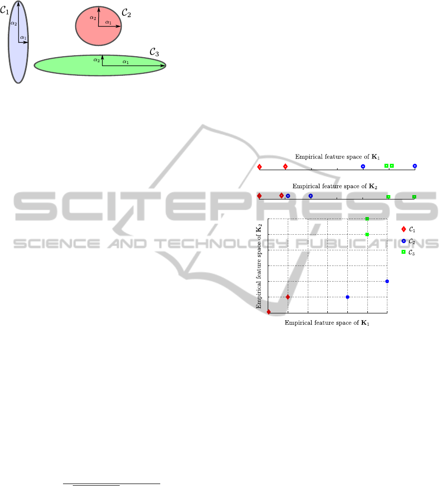
Figure 1: Representation of a toy dataset with different local
neighbourhoods.
and the ideal kernel, as follows:
α
∗
i
= argmax
α
i
A
c
(K
α
i
, K
∗
i
). (4)
In this paper, the parameters are adjusted by the
use of CKTA and a multi-scale kernel, as previously
done in (P
´
erez-Ortiz et al., 2013). Once that the mul-
tiple kernel parameters are learnt for each decomposi-
tion, the multiple outputs have to be combined into a
single prediction vector. As said, this can be done
using one model per decomposition and fusing the
predictions, or, alternatively, combining the multiple
kernel matrices into one and solving it with a sin-
gle model. This latter option is explored in this pa-
per by means of multiple kernel learning techniques.
The multiple kernel learning problem is formulated
in such a way that it can be solved by means of a
Quadratic Programming (QP) problem optimiser.
The solution of this QP problem will result in
a kernel matrix defining the optimal feature space
for the whole considered problem (which will be af-
terwards used by the classification method). More
specifically, we optimise a convex combination of
kernel matrices K
δ
=
∑
K
i=1
δ
i
K
i
(with δ
i
≥ 0 and
∑
p
i=1
δ
i
= 1), where, as said, each matrix K
i
is associ-
ated to a different decomposition D
i
and will be opti-
mised separately from the rest by the gradient ascent
methodology previously mentioned (obtaining thus a
vector of optimal kernel parameters α
i
). This optimi-
sation problem can also be formulated using the no-
tion of CKTA:
max
δ∈M
K
δ
c
, K
∗
c
F
q
K
δ
c
, K
δ
c
F
h
K
∗
c
, K
∗
c
i
F
,
where M = {δ : ||δ||
2
= 1}, and K
δ
c
is the centered
version of K
δ
. The QP optimization problem associ-
ated is solved as in (Cortes et al., 2012).
As outlined in (Yan et al., 2010) taking the un-
weighted sum of p base kernels is equivalent to taking
the Cartesian product of the empirical feature spaces
associated with the base kernels (being the empirical
feature space an Euclidean isomorphic space to the
feature space). Furthermore, taking the weighted sum
is equivalent to taking the Cartesian product of the
base empirical feature spaces scaled with δ
1
, . . . , δ
K
.
As done in (Yan et al., 2010), we illustrate the geo-
metrical interpretation of taking the unweighted sum
of two kernels in Figure 2 for a 3-class ordinal prob-
lem (the decompositions being C
1
vs. {C
2
, C
3
} and
{C
1
, C
2
} vs. C
3
). Note that for the sake of visualisa-
tion we assume that both empirical feature spaces are
1-dimensional while in practice both spaces can be
up to N-dimensional. It can be appreciated from this
Figure that in the combined empirical feature space
the classes can be perfectly separated (although this
is not so for the decomposed problems).
−3 −2 −1 0 1 2 3
0
−3 −2 −1 0 1 2 3
0
−3 −2 −1 0 1 2 3
−3
−2
−1
0
1
2
3
Figure 2: Geometrical interpretation of taking the sum of
two kernels. The bottom part of the plot represents the em-
pirical feature space of K
1
+ K
2
.
4 EXPERIMENTS
The proposed methodologies have been tested con-
sidering the Support Vector Ordinal Regression with
Implicit Constraints (SVORIM) (Chu and Keerthi,
2007). 8 benchmark ordinal regression datasets have
been used for the analysis. Some of the ordinal regres-
sion benchmark datasets (stock and machine) pro-
vided by Chu et. al (Chu and Ghahramani, 2005) were
considered, because they are widely used in the ordi-
nal regression literature (Sun et al., 2010; Chu and
Keerthi, 2007). These two datasets are originally re-
gression tasks. To turn regression into ordinal classi-
fication, the target variable is discretised into K bins
(representing the number of classes, in this case we
choose K = 10), with equal frequency for each bin
(i.e. the size of the bins is adjusted to have the same
number of patterns for each class). Table 2 shows
the characteristics of the datasets used for the experi-
ments.
LearningKernelLabelDecompositionsforOrdinalClassificationProblems
221

Table 2: Characteristics of the benchmark datasets used, or-
dered by the number of classes
Dataset N d K Class distr.
contact-lenses 24 6 3 (15, 5, 4)
pasture 36 25 3 (12, 12, 12)
SWD 1000 10 4 (32, 352, 399, 217)
eucalyptus 736 91 5 (180, 107, 130, 214, 105)
LEV 1000 4 5 (93, 280, 403, 197, 27)
automobile 205 71 6 (3, 22, 67, 54, 32, 27)
machine 209 7 10 (21, 21, 21, 21, 21,
21, 21, 21, 21, 20)
stock 700 9 10 (70, 70, 70, 70, 70,
70, 70, 70, 70, 70)
In the experiments, the ordinal reformulation of
the SVM pardigm optimising the uni-scale kernel pa-
rameters through cross-validation (SVORIM) is com-
pared to the ordinal label decomposition approach,
using both uni-scale and multi-scale kernel learning
(UOKL and MSOKL, respectively).
For ordinal classification, the most common eval-
uation measures are the Mean absolute error (MAE)
and the accuracy ratio (Acc) (Guti
´
errez et al., 2012).
The MAE measure is an evaluation metric used when
the costs of different misclassification errors vary
markedly (as in the ordinal classification learning set-
ting). It is defined as:
MAE =
1
N
N
∑
i=1
|y
i
− ˆy
i
|, (5)
where ˆy
i
is the label predicted for x
i
. MAE values
range from 0 to K − 1 (Baccianella et al., 2009).
Regarding the experimental setup, a holdout strat-
ified technique was applied to divide the datasets 30
times, using 75% of the patterns for training and the
remaining 25% for testing. The partitions were the
same for all methods and one model was obtained and
evaluated (in the test set), for each split. Finally, the
results are taken as the mean and standard deviation
of the measures over the 30 test sets.
The parameters of each algorithm are chosen us-
ing a nested cross-validation considering only the
training set (specifically, a 5-fold method). The cross-
validation criteria (the measure used to select the
best parameter combination) is the MAE. For cross-
validation, the kernel width was selected within the
values {10
−3
, 10
−2
, . . . , 10
3
}, as well as the cost pa-
rameter (C) associated with SVORIM. Note that for
all of the methods tested, the C parameter is selected
by cross-validation.
4.1 Results
Table 3 shows the mean test results for the 8 ordinal
datasets considered in terms of Acc and MAE. The
best results are in bold face and the second ones in
italics. First of all, it can be appreciated from this Ta-
ble that the use of the proposed methodology helps to
improve both evaluation metrics. For all datasets, the
results using multi-scale kernel learning based on dif-
ferent binary decompositions (MSOKL) improves the
original results of SVORIM obtained through cross-
validation. Furthermore, it is also noticeable that the
use of a uni-scale kernel (UOKL) is not suitable for
this strategy (except in LEV and SWD), as it usually
obtains worse results than SVORIM. This result is due
to the fact that learning and combining uni-scale ker-
nels significantly restricts the solution space. The in-
dependent information of the binary decompositions
needs a more flexible kernel to be correctly repre-
sented.
Table 3: Results obtained for the ordinal datasets.
Dataset Method Acc MAE
SWD
SVORIM 56.87 ± 2.81 0.447 ± 0.029
UOKL 56.85 ± 3.09 0.447 ± 0.031
MSOKL 57.96 ± 2.55 0.432 ± 0.027
automobile
SVORIM 66.79 ± 6.58 0.402 ± 0.090
UOKL 52.18 ± 9.13 0.635 ± 0.135
MSOKL 73.85 ± 6.46 0.342 ± 0.076
contact-lenses
SVORIM 63.89 ± 12.44 0.478 ± 0.189
UOKL 63.33 ± 6.78 0.533 ± 0.068
MSOKL 71.11 ± 10.66 0.444 ± 0.192
eucalyptus
SVORIM 64.11 ± 3.14 0.393 ± 0.032
UOKL 32.97 ± 5.28 0.936 ± 0.075
MSOKL 65.11 ± 2.96 0.365 ± 0.032
LEV
SVORIM 62.84 ± 2.40 0.407 ± 0.027
UOKL 63.47 ± 2.66 0.403 ± 0.028
MSOKL 62.69 ± 2.46 0.409 ± 0.026
machine
SVORIM 36.53 ± 5.67 0.930 ± 0.129
UOKL 34.75 ± 5.54 1.029 ± 0.116
MSOKL 38.47 ± 5.01 0.897 ± 0.097
pasture
SVORIM 66.30 ± 9.89 0.337 ± 0.099
UOKL 33.33 ± 0.00 0.667 ± 0.000
MSOKL 84.81 ± 10.71 0.152 ± 0.107
stock
SVORIM 76.93 ± 1.97 0.238 ± 0.022
UOKL 76.00 ± 2.03 0.250 ± 0.022
MSOKL 78.43 ± 1.93 0.221 ± 0.020
4.2 Discussion
In order to better justify the results obtained, Ta-
ble 4 shows the δ values obtained for each dataset
(i.e. the weight assigned to each kernel matrix by
the kernel learning algorithm). Note that there are
K −1 matrices and weights (from the decompositions
in Table 1) plus the original classification problem
(δ
0
). As outlined in the previous section, the proposal
was successful as it outperforms the base algorithm
(SVORIM). It can be seen that usually multiple ker-
NCTA2014-InternationalConferenceonNeuralComputationTheoryandApplications
222

Table 4: Weights of the convex combination obtained for the different datasets and decompositions.
Dataset Weight parameters obtained [δ
1
, . . . , δ
K−1
, δ
O
]
automobile [0.0000 0.0142 0.2200 0.0538 0.1950 0.5169]
SWD [0.0140 0.1763 0.0857 0.7239]
eucalyptus [0.0191 0.3745 0.1235 0.0144 0.4685]
contact-lenses [0.1259 0.1452 0.7290]
LEV [0.0000 0.0202 0.1208 0.0204 0.8386]
machine [0.2172 0.0204 0.0075 0.0209 0.0044 0.0104 0.0024 0.0115 0.5043 0.2008]
stock [0.0172 0.0000 0.1546 0.0000 0.0000 0.0000 0.0351 0.0000 0.0002 0.7928]
pasture [0.1447 0.1790 0.6763]
nel matrices are combined. For some datasets such
as LEV and stock, there are decomposition with a 0
weight, meaning that they are not useful for the learn-
ing task. Even taking into account that the last decom-
position has been chosen to be the original learning
problem, the weight of this kernel matrix is very low
for some of the datasets (e.g. machine and eucalyptus
datasets). This is important, because it means that the
original problem can be successfully combined with
other information (the decompositions learnt) in or-
der to improve the overall classification.
In order to explore this last result in depth,
we studied several complexity measures (Ho and
Basu, 2002) of the decomposed problems to analyse
whether there exist some relation between the kernel
matrices presenting the highest weights and the com-
plexity of these decomposed learning problems (the
results obtained can be seen in Table 5). The com-
plexity measures chosen in this case are the maximum
fisher’s discriminant ratio (F1), the maximum (indi-
vidual) feature efficiency (L3), the minimised sum of
the error distance of a linear classifier (L1) and the
fraction of points in the class boundary (N1). Decom-
posed problems with highter F1 and F3 and lower L1
and N1 are the ones with lower complexity. Given
that these measures are designed for binary classifica-
tion, the original problem D
0
is not included. It can
be seen that for the case of automobile the decom-
positions associated to a lower complexity (i.e. D
1
and D
2
which present high values for F1 and F3 and
low values for L1 and N1) are the ones with a lower
weight. This is also applicable for eucalyptus. Fur-
thermore, it can be seen that the most complex de-
compositions (D
3
and D
5
for automobile and D
2
and
D
3
for eucalyptus) present relatively high weights.
On the other hand, this is not such a straightforward
conclusion for the machine dataset. In this case, it
can be observed that D
9
(which can be considered
as the simplest problem for 3 of the 4 selected met-
rics) presents the highest weight. In order to anal-
yse this, we computed the angle between the vector
of parameters learnt by the algorithm for all the de-
compositions of this dataset (note that this angle will
provide information about the direction of the vec-
tors, but not the magnitude of these). The angles ob-
tained for α
9
(decomposition D
9
) with respect to the
rest of decompositions is relatively low (an average
angle of 25 degrees). This could indicate that this
vector of parameters represents properly the ones ob-
tained for the rest of decompositions. However, for
the case of α
1
(where D
1
also presents a high weight)
the mean angle with respect to the other vectors is 51
degrees. This could indicate that D
1
represents a rela-
tion between the features that greatly differs from the
rest and helps to improve the goodness of the kernel
matrix. Although these results may not be conclu-
sive, they indicate that there exist a relation between
the final weights and the nature of the different de-
composed problems, which could be studied in future
work.
5 CONCLUSIONS
This paper proposes a novel way of applying ker-
nel learning for multiclass datasets, where the orig-
inal problem is decomposed in binary subproblems
and one kernel matrix is learnt for each one. Then,
all matrices are combined by using a multiple kernel
learning technique. This algorithm has the benefit of
adapting the kernel matrix individually for each class
(or subproblem), but combining all the information in
one single model, without having to learn several in-
dependent models and specifying how to reach a con-
sensus from their decision values.
The algorithm is applied to ordinal classification
problems. When combined with the support vector
ordinal regression with implicit constraints method,
the results seem to confirm that this kind of learn-
ing leads to improve generalisation results. The al-
gorithm detects the importance of the different ker-
nel matrices, assigning accordingly their weights. An
analysis of the complexity of the binary subtasks con-
firms these findings. For future work, we will study
LearningKernelLabelDecompositionsforOrdinalClassificationProblems
223

Table 5: Complexity measures computed for the differ-
ent decompositions of automobile, eucalyptus and machine
datasets.
D
i
Weights Complexity measures
automobile δ
i
F1 F3 L1 N1
D
1
0.0000 13.41 0.99 0.04 0.05
D
2
0.0142 13.04 0.46 0.29 0.15
D
3
0.2200 0.83 0.22 0.43 0.22
D
4
0.0538 2.93 0.26 0.58 0.28
D
5
0.1950 0.96 0.57 0.33 0.16
eucalyptus δ
i
F1 F3 L1 N1
D
1
0.0191 2.72 0.17 0.40 0.20
D
2
0.3745 1.48 0.21 0.51 0.24
D
3
0.1235 1.80 0.10 0.58 0.31
D
4
0.0144 2.72 0.30 0.34 0.22
machine δ
i
F1 F3 L1 N1
D
1
0.2172 0.66 0.57 0.20 0.17
D
2
0.0204 0.89 0.43 0.42 0.19
D
3
0.0075 0.82 0.39 0.61 0.23
D
4
0.0209 0.97 0.30 0.77 0.26
D
5
0.0044 1.01 0.22 0.74 0.23
D
6
0.0104 1.13 0.22 0.63 0.23
D
7
0.0024 1.45 0.37 0.50 0.12
D
8
0.0115 1.80 0.45 0.39 0.09
D
9
0.5043 2.04 0.80 0.25 0.05
the computational complexity of our method (as ker-
nel learning methods usually present a high computa-
tional cost in this sense) and try to alleviate it via the
Nymstr
¨
on method for approximating Gram matrices
(Drineas and Mahoney, 2005).
ACKNOWLEDGEMENTS
This work has been subsidized by the TIN2011-22794
project of the Spanish Ministerial Commission of Sci-
ence and Technology (MICYT), FEDER funds and
the P11-TIC-7508 project of the “Junta de Andaluc
´
ıa”
(Spain).
REFERENCES
Baccianella, S., Esuli, A., and Sebastiani, F. (2009). Evalu-
ation measures for ordinal regression. In Proceedings
of the Ninth International Conference on Intelligent
Systems Design and Applications (ISDA 09), pages
283–287, Pisa, Italy.
Cardoso, J. S. and da Costa, J. F. P. (2007). Learning to clas-
sify ordinal data: The data replication method. Jour-
nal of Machine Learning Research, 8:1393–1429.
Chapelle, O., Vapnik, V., Bousquet, O., and Mukherjee,
S. (2002). Choosing multiple parameters for support
vector machines. Machine Learning, 46(1-3):131–
159.
Chu, W. and Ghahramani, Z. (2005). Gaussian processes
for ordinal regression. Journal of Machine Learning
Research, 6:1019–1041.
Chu, W. and Keerthi, S. S. (2007). Support vector ordinal
regression. Neural Computation, 19(3):792–815.
Cortes, C., Mohri, M., and Rostamizadeh, A. (2012).
Algorithms for learning kernels based on centered
alignment. Journal of Machine Learning Research,
13:795–828.
Cortes, C. and Vapnik, V. (1995). Support-vector networks.
Machine Learning, 20(3):273–297.
Cristianini, N., Kandola, J., Elisseeff, A., and Shawe-
Taylor, J. (2002). On kernel-target alignment. In Ad-
vances in Neural Information Processing Systems 14,
pages 367–373. MIT Press.
Drineas, P. and Mahoney, M. W. (2005). On the
nyström method for approximating a gram ma-
trix for improved kernel-based learning. J. Mach.
Learn. Res., 6:2153–2175.
Frank, E. and Hall, M. (2001). A simple approach to ordi-
nal classification. In Proc. of the 12th Eur. Conf. on
Machine Learning, pages 145–156.
Friedrichs, F. and Igel, C. (2005). Evolutionary tuning of
multiple svm parameters. Neurocomputing, 64:107–
117.
Guti
´
errez, P. A., P
´
erez-Ortiz, M., Fernandez-Navarro,
F., S
´
anchez-Monedero, J., and Herv
´
as-Mart
´
ınez, C.
(2012). An Experimental Study of Different Ordi-
nal Regression Methods and Measures. In 7th Inter-
national Conference on Hybrid Artificial Intelligence
Systems (HAIS), volume 7209 of Lecture Notes in
Computer Science, pages 296–307.
Ho, T. K. and Basu, M. (2002). Complexity measures of su-
pervised classification problems. IEEE Trans. Pattern
Anal. Mach. Intell., 24(3):289–300.
Hsu, C.-W. and Lin, C.-J. (2002). A comparison of methods
for multi-class support vector machines. IEEE Trans-
action on Neural Networks, 13(2):415–425.
Igel, C., Glasmachers, T., Mersch, B., Pfeifer, N., and
Meinicke, P. (2007). Gradient-based optimization of
kernel-target alignment for sequence kernels applied
to bacterial gene start detection. IEEE/ACM Trans.
Comput. Biol. Bioinformatics, 4(2):216–226.
Li, L. and Lin, H.-T. (2007). Ordinal Regression by Ex-
tended Binary Classification. In Advances in Neural
Inform. Processing Syst. 19.
P
´
erez-Ortiz, M., Guti
´
errez, P., Cruz-Ram
´
ırez, M., S
´
anchez-
Monedero, J., and Herv
´
as-Mart
´
ınez, C. (2013). Ker-
nelizing the proportional odds model through the em-
pirical kernel mapping. In Rojas, I., Joya, G., and
Gabestany, J., editors, Advances in Computational In-
telligence, volume 7902 of Lecture Notes in Computer
Science, pages 270–279. Springer Berlin Heidelberg.
P
´
erez-Ortiz, M., Guti
´
errez, P. A., S
´
anchez-Monedero, J.,
and Herv
´
as-Mart
´
ınez, C. (2013). Multi-scale Sup-
port Vector Machine Optimization by Kernel Target-
Alignment. In European Symposium on Artificial
NCTA2014-InternationalConferenceonNeuralComputationTheoryandApplications
224

Neural Networks, Computational Intelligence and
Machine Learning (ESANN), pages 391–396.
Ramona, M., Richard, G., and David, B. (2012). Multi-
class feature selection with kernel gram-matrix-based
criteria. IEEE Trans. Neural Netw. Learning Syst.,
23(10):1611–1623.
Shashua, A. and Levin (2003). Advances in Neural Infor-
mation Processing Systems, volume 15, chapter Rank-
ing with large margin principle: Two approaches,
pages 937–944. MIT Press, Cambridge.
Sun, B.-Y., Li, J., Wu, D. D., Zhang, X.-M., and Li, W.-B.
(2010). Kernel discriminant learning for ordinal re-
gression. IEEE Transactions on Knowledge and Data
Engineering, 22:906–910.
Vapnik, V. N. (1998). Statistical learning theory. Wiley, 1
edition.
Waegeman, W. and Boullart, L. (2009). An ensemble of
weighted support vector machines for ordinal regres-
sion. International Journal of Computer Systems Sci-
ence and Engineering, 3(1):1–7.
Yan, F., Mikolajczyk, K., Kittler, J., and Tahir, M. A.
(2010). Combining multiple kernels by augmenting
the kernel matrix. In Proc. of the 9th International
Workshop on Multiple Classifier Systems (MCS), vol-
ume 5997, pages 175–184. Springer.
LearningKernelLabelDecompositionsforOrdinalClassificationProblems
225
