
Predictive Modeling in 400-Metres Hurdles Races
Krzysztof Przednowek
1
, Janusz Iskra
2
and Karolina H. Przednowek
1
1
Faculty of Physical Education, University of Rzeszow, Rzeszów, Poland
2
Faculty of Physical Education, Academy of Physical Education in Katowice, Katowice, Poland
Keywords: Hurdling, Shrinkage Regression, Artificial Neural Networks, Sport Prediction.
Abstract: The paper presents the use of linear and nonlinear multivariable models as tools to predict the results of
400-metres hurdles races in two different time frames. The constructed models predict the results obtained
by a competitor with suggested training loads for a selected training phase or for an annual training cycle.
All the models were constructed using the training data of 21 athletes from the Polish National Team. The
athletes were characterized by a high level of performance (score for 400 metre hurdles: 51.26±1.24 s). The
linear methods of analysis include: classical model of ordinary least squares (OLS) regression and
regularized methods such as ridge regression, LASSO regression. The nonlinear methods include: artificial
neural networks as multilayer perceptron (MLP) and radial basis function (RBF) network. In order to
compare and choose the best model leave-one-out cross-validation (LOOCV) is used. The outcome of the
studies shows that Lasso shrinkage regression is the best linear model for predicting the results in both
analysed time frames. The prediction error for a training period was at the level of 0.69 s, whereas for the
annual training cycle was at the level of 0.39 s. Application of artificial neural network methods failed to
correct the prediction error. The best neural network predicted the result with an error of 0.72 s for training
periods and 0.74 for annual training cycle. Additionally, for both training frames the optimal set of
predictors was calculated.
1 INTRODUCTION
Today we have a very high level of sport. The
competitors and coaches have been looking for new
solutions to optimize the training process. One of
way is using the advances mathematical methods in
planning the training loads. Advanced mathematical
models include among others regularized linear
models and intelligent computational methods.
Those models facilitate description of training,
which is a complex process, help to notice
interrelations between the training load and the final
result.
Sports prediction involves many aspects
including predicting sporting talent (Papić et al.,
2009, Roczniok et al., 2013) or the prediction of
performance results (Maszczyk et al., 2011,
Przednowek and Wiktorowicz, 2013). Models
predicting sports scores, taking into account the
seasonal statistics of each team, are also constructed
(Haghighat et al., 2013). The present work focuses
on predicting outcomes in terms of sports training.
The use of regression models in athletics was
described by Maszczyk et al., (2011), where the
model implementing the prediction of results in a
javelin throw was presented. The constructed model
was used as a tool to support the choice and
selection of prospective javelin throwers. On the
basis of the selected set of input variables the
distance of a javelin throw was predicted. The
models presented were classic multiple regression
models, and to select input variables Hellwig’s
method was used.
Another application used in walking races was
regressions estimating the levels of the selected
physiological parameters and the results over
distances of 5, 10, 20 and 50 km (Drake and James,
2009). Calculated models were used to develop
nomograms. The regressions applied were the
classical OLS models, and the coefficient R
2
was
chosen for the quality criterion. The study included
45 men and 23 women. The amount of registered
data was changed depending on the implemented
task and ranged from 21 to 68 models.
Chatterjee et al., (2009) have calculated a
nonlinear regression equation to predict the maximal
aerobic capacity of footballers. The data, on the
137
Przednowek K., Iskra J. and H. Przednowek K..
Predictive Modeling in 400-Metres Hurdles Races.
DOI: 10.5220/0005082201370144
In Proceedings of the 2nd International Congress on Sports Sciences Research and Technology Support (icSPORTS-2014), pages 137-144
ISBN: 978-989-758-057-4
Copyright
c
2014 SCITEPRESS (Science and Technology Publications, Lda.)

basis of which the models were calculated, came
from 35 young players aged from 14 to 16. The
experiment was to verify the use of the test of 20-m
MST (Multi Stage Shuttle Run Test) in assessing the
performance of
.
Roczniok et al., (2013) used a regression
equation to identify the talent of young hockey
players. The study involved 60 boys aged between
15 and 16, who participated in selection camps. The
applied regression model classified individual
candidates for future training based on selected
parameters of the player. The classification method
used was logistic regression.
A group of nonlinear predictive models used in
sport also supplement the selected methods of ’data
mining’. Among them a significant role is played by
fuzzy expert systems. Practical application of such a
system has been described in the work by Papić et
al. (2009). The presented system used the knowledge
of experts in the field of sport, as well as the data
obtained as a result of a number of motor tests. The
model based on the candidate’s data suggested the
most suitable sport. This tool was designed to help
to search for prospective sports talents.
Previous studies also concern the widespread use
of artificial neural networks in sports prediction
(Haghighat et al., 2013). Artificial neural networks
are used to predict sporting talent, to identify
handball players’ tactics or to analyze the
effectiveness of the training of swimmers (Pfeiffer
and Hohmann, 2012). Numerous studies show the
application of neural networks in various aspects of
sports training (Ryguła, 2005, Silva et al., 2007,
Maszczyk et al., 2012). These models support the
selection of sports, practice control or the planning
of training loads.
The main purpose of the research was
verification of artificial neural methods and
regularized linear models (shrinkage regression) in
prediction result in 400-metres hurdles for two
different time frames. The verification was carried
out based on training data of athletes running the
400-metres hurdles and featuring a very high level
of sport abilities.
2 MATERIAL AND METHODS
The analysis included 21 Polish hurdlers aged
22.25±1.96 years participating in competitions from
1989 to 2011. The athletes had a high sport level
(the result over 400-metres hurdles: 51.26±1.24 s).
They were the part of the Polish National Athletic
Team Association representing Poland at the
Olympic Games, World and European
Championships in junior, youth and senior age
categories. The best result over 400-metres hurdles
in the examined group amounted to 48.19 s.
Table 1: Description of the variables used to construct the
models.
Variable
Description
Training
period
Annual
cycle
y - Expected 500 m sprint (s)
- y
Expected result on 400-metres
hurdles (s)
x
1
x
1
Age (years)
x
2
x
2
Body mass index
x
3
- Current 500 m sprint (s)
- x
3
Current result on 400-metres
hurdles (s)
x
4
- Period GPP*
x
5
- Period SPP*
x
6
x
4
Maximal speed (m)
x
7
x
5
Technical speed (m)
x
8
x
6
Technical and speed exercises
(m)
x
9
x
7
Speed endurance (m)
x
10
x
8
Specific hurdle endurance (m)
x
11
x
9
Pace runs (m)
x
12
x
10
Aerobic endurance (m)
x
13
x
11
Strength endurance I (m)
x
14
x
12
Strength endurance II (n)
x
15
x
13
General strength of lower limbs
(kg)
x
16
x
14
Directed strength of lower limbs
(kg)
x
17
x
15
Specific strength of lower limbs
(kg)
x
18
x
16
Trunk strength (amount)
x
19
x
17
Upper body strength (kg)
x
20
x
18
Explosive strength of lower limbs
(amount)
x
21
x
19
Explosive strength of upper limbs
(amount)
x
22
x
20
Technical exercises – walking
pace (min)
x
23
x
21
Technical exercises – running
pace (min)
x
24
x
22
Runs over 1-3 hurdles (amount)
x
25
x
23
Runs over 4-7 hurdles(amount)
x
26
x
24
Runs over 8-12 hurdles (amount)
x
27
x
25
Hurdle runs in varied rhythm
(amount)
*-in accordance with the rule of introducing a qualitative variable
of a “training type” with the value of general preparation period,
specific preparation period and competitive period was replaced
with two variables x
4
and x
5
holding the value of 1 or 0.
The collected material allowed for the analysis of
144 training plans used in one of the three periods
during the annual cycle of training, lasting three
icSPORTS2014-InternationalCongressonSportSciencesResearchandTechnologySupport
138

months each. The annual training cycle is divided
into three equal periods: general preparation, special
preparation and the starting period. In the analysis of
training periods, 28 variables were used, including
27 independent variables and 1 dependent variable
(Table 1).
Another examined time interval was the
one-year training cycle, in which the training loads
were considered as sums of the given training means
used throughout the whole macrocycle. In the one-
year training cycle, 25 variables were specified. In
order to develop models for the one-year training
cycle, a total of 48 standard training plans were
used.
2.1 Regularized Linear Regression
We are considering the problem of constructing a
multivariable (multiple) regression model for the set
of multiple inputs
,1,…,, and the one output
Y. The input variables
are called predictors,
whereas the output variable Y – a response. We have
assumed that it is a linear regression model in the
parameters. In OLS regression a popular method of
least squares is used (Hastie, et al. 2009; Bishop,
2006), in which weights are calculated by
minimizing the sum of the squared errors. The
criterion of performance
takes the form:
(1)
where
,
, are unknown weights (parameters) of
the model.
In ridge regression by Hoerl and Kennard (1970)
the criterion of performance includes a penalty for
increased weights and takes the form:
,
(2)
Parameter 0 decides the size of the penalty: the
greater the value λ the bigger the penalty; for 0
ridge regression is reduced to OLS regression.
LASSO regression by Tibshirani (1996),
similarly to ridge regression, adds to the criterion of
performance penalty, where instead of L
2
the norm
L
1
is used i.e. the sum of absolute values:
,
(3)
To solve this regression an implementation of the
popular LARS algorithm was used (least angle
regression) (Efron et al., 2004). In the applied
algorithm the penalty is decided by s parameter from
the section from 0 to 1. The parameter is the fraction
of the penalty used in the LASSO. This regression is
also used for the selection of input variables.
Regularized linear models were implemented in
GNU R software programming language with
additional packets.
2.2 Artificial Neural Network
In order to build the predictive model, artificial
neural networks (ANN) were also used. Two types
of ANNs were applied: a multi-layer perceptron
(MLP) and networks with radial basis functions
(RBF) (Bishop, 2006).
The multi-layer perceptron is the most common
type of neural network. In 3-layer multiple-input-
one-output network the calculation of the output is
performed in feed-forward architecture. Network
teaching was implemented by the BFGS (Broyden-
Fletcher-Goldfarb-Shanno) algorithm, which is a
strong second-order algorithm. During MLP training
exponential and hyperbolic tangent function were
used as the activation functions of hidden neurons.
All the analysed networks have only one hidden
layer.
The problem with MLP network is that it can be
overtrained which means good fitting to data, but
poor predictive (generalization) ability. To avoid this
the number m of hidden neurons, which is a free
parameter, should be determined to give the best
predictive performance.
In the RBF network we use the concept of radial
basis function. The model of linear regression (5) is
extended by considering linear combinations of
nonlinear functions of the predictors in the form:
(4)
where
,…,
is a vector of so called
basis functions. If we use nonlinear basis functions,
we get the nonlinear model which is, however, a
linear function of parameters
j
w
. The feature of
RBF network is the fact that the hidden neuron
performs a radial basis function.
To implement MLP and RBF the Statistica 10
program was used along with the Automatic
Statistica Neural Network.
PredictiveModelingin400-MetresHurdlesRaces
139

2.3 Evaluation of Models
In order to select the best model the method of
cross-validation (CV) (Arlot and Celisse, 2010) was
applied. In this method, the data set is divided into
two subsets: learning and testing (validation). The
first of them is used to build the model, and the
second to evaluate its quality. In this article, due to
the small amount of data, leave-one-out cross-
validation, (LOOCV) was chosen, in which a test set
is composed of a selected pair of data (x
i
, y
i
), and the
number of tests is equal to the number of data n. As
an indicator of the quality of the model the root of
the mean square error was calculated from formula:
1
(5)
where: n – total number of patterns,
– the output
value of the model built in the i-th step of cross-
validation based on a data set containing no testing
pair (x
i
, y
i
),
– Root Mean Square Error.
3 RESULTS AND DISCUSSION
3.1 Prediction in Training Periods
Result prediction concerning the training period for
400-metres hurdle race involves a defined training
status indicator, since it is technically impossible to
use the running test in 400-metres hurdles within
each of the analysed annual cycle periods.
Therefore, as the training status indicator, the result
of a race over a flat distance of 500 m in the
particular periods was assumed. The correlation
between the result of 500 m and 400-metres hurdles
within the competition period is very strong
(r
xy
=0,84); apart from that, it demonstrates statistical
significance at the level of α=0,001, confirming the
validity of assumption of the 500 m race result as a
dependent variable in the course of prediction
models development.
The development of a predictive model makes it
possible to check how the suggested training affects
the final result. The basic model is OLS regression,
for which the cross-validation error was at the level
of
0.74s.
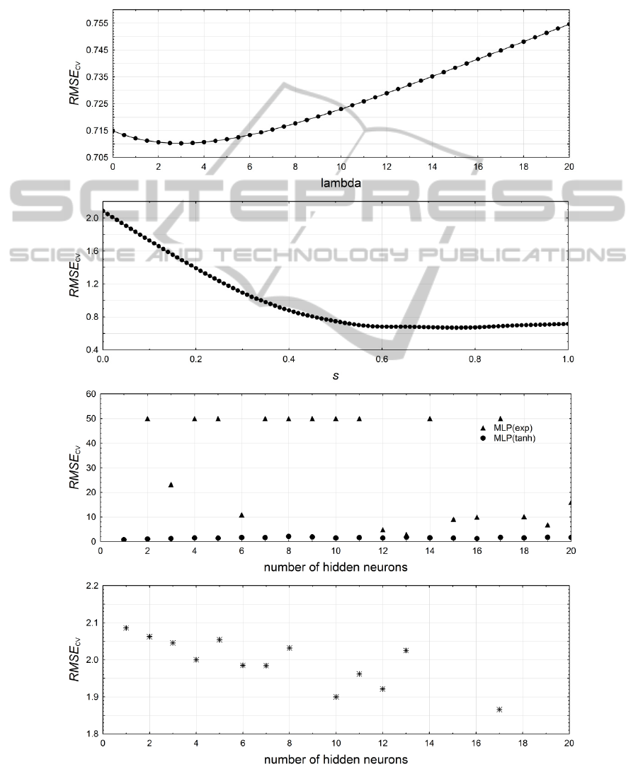
In ridge regression, the λ parameter is chosen; it
determines the additional penalty associated with the
regression coefficients. In the study, the dependency
between the prediction error and the parameter λ
changing from 0 to 20 in steps of 0.1 (Fig. 1a) was
determined. The smallest error is generated for the
model in which the parameter
3. The cross-
validation error for the optimal ridge regression is
0,71 s. It was also noted that at the initial stage of
model optimization, along with the increase of
penalty parameter, the prediction error slightly
decreases, and after reaching the minimum, it
increases up to the level of approx. 0,8 s.
In the LASSO model, the s parameter is chosen;
its value ranges from 0 to 1 and it determines the
imposed penalty. A graph showing the relationship
between the s parameter values and the prediction
error
was drafted (Fig. 1b).
The error generated by the optimal LASSO
model (0,76) was at the level of 0,67 s. From
the determined coefficients (Tab. 2) it follows, that
the variables x
2
, x
5
, x
8
, x
11
, x
15
, x
16
, x
23
, x
25
are not
taken into account in the prediction task in terms of
training periods (coefficients equal to 0).
Table 2: Coefficients of linear models and error results
- training periods.
Regression OLS Ridge Lasso
Intercept 1,75e+01 2,20e+01 15,254
x
1
-6,43e-02 -8,12e-02 -0,058
x
2
-1,83e-02 -4,35e-02
0
x
3
7,50e-01 6,96e-01 0,776
x
4
4,85e-01 5,11e-01 0,562
x
5
-9,79e-02 -4,03e-02
0
x
6
1,28e-04 1,29e-04 1,86e-05
x
7
1,44e-04 1,44e-04 9,10e-05
x
8
-7,75e-05 -6,21e-05
0
x
9
2,43e-07 6,38e-08 6,21e-07
x
10
-9,04e-05 -8,98e-05 -8,33e-05
x
11
-2,67e-06 -2,39e-06
0
x
12
1,24e-06 1,25e-06 5,73e-07
x
13
-1,51e-05 -1,52e-05 -1,41e-05
x
14
-4,47e-05 -4,49e-05 -2,12e-05
x
15
5,88e-07 1,65e-07
0
x
16
4,77e-06 2,93e-06
0
x
17
1,31e-06 2,58e-06 1,26e-06
x
18
4,19e-06 3,48e-06 2,14e-06
x
19
-3,00e-05 -2,93e-05 -1,05e-05
x
20
-1,42e-03 -1,35e-03 -0,001
x
21
-3,28e-04 -4,23e-04 -0,0004
x
22
1,13e-03 1,34e-03 0,0006
x
23
3,94e-04 4,74e-04
0
x
24
-3,82e-03 -3,78e-03 -0,0019
x
25
-6,10e-04 -9,13e-04
0
x
26
-9,59e-04 -1,29e-03 -0,0007
x
27
5,68e-04 6,34e-04 0,0003
[s]
0,74 0,71
0,67
The eliminated training means belong to the group
of “targeted” ones. The results confirm thus the
views prevailing among sport researchers, that in
high-qualified training those exercises should be
icSPORTS2014-InternationalCongressonSportSciencesResearchandTechnologySupport
140
restricted, and the coach should concentrate on
special training (Iskra, 2013).
Calculation of the best neural model performing
the task of result prediction in terms of training
period amounts to determination of the number of
neurons in the hidden layer and to selection of the
optimal function of hidden layer neurons activation.
Therefore, the dependency between prediction
error and the number of neurons in the hidden layer
for each of the analysed networks was determined
(Fig. 1cd).
a)
b)
c)
d)
Figure 1: Predictive error for training period.
PredictiveModelingin400-MetresHurdlesRaces
141
a)
b)
c)
d)
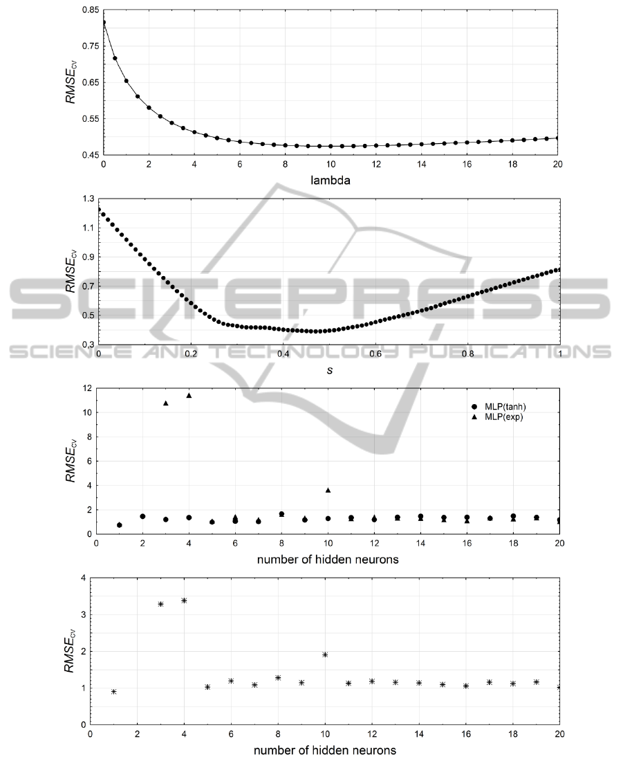
Figure 2: Predictive error for annual training cycle.
The first type of network was a multilayer
perceptron with the function of hyperbolic tangent
activation. Neural networks consisting of from 1 to
20 neurons in the hidden layer were subjected to
examination. It can be noted that the smallest
prediction error is obtained for 1 neuron in the
hidden layer (Fig. 1c). Prediction error for the
optimalmodel is 0.73 s, and it does not improve the
icSPORTS2014-InternationalCongressonSportSciencesResearchandTechnologySupport
142

result obtained by the LASSO regression model.
Another network is the MLP network with
exponential function. The optimal model for
exponential activation function includes also 1
neuron in the hidden layer. The prediction error
(
0.72) is smaller in comparison to
hyperbolic tangent function, but it is greater than the
LASSO regression model. Similar to MLP networks,
RBF network was also subjected to cross-validation.
The results are presented in form of a graph, where
the prediction error values are shown (Fig. 1d).
The optimal RBF model executing the
considered task includes 12 neurons in the hidden
layer and generates the error of
1.9 s.
Errors generated by the RBF network are the
greatest among the analysed models.
3.2 Prediction in Annual Training
Cycle
OLS model is the basic method applied while
seeking optimal solutions for predicting outcome in
the annual cycle. The following regression performs
this task with error
0.81 s, all the
coefficients are different from zero (Table 3), which
means that all the variables form a final result.
The analysed ridge models are regressions for
the parameter λ equal from 1 to 20 (Fig. 2a). The
best model was obtained for the parameter 10.
A prediction error generated by the best ridge
regression is
0.47 s. Application of this
method has improved by almost a half the capacity
of prediction results compared to OLS regression.
Ridge regression coefficients, as in the classical
model, are different from zero (Table 3), so all the
input variables are involved in the formation of the
projected result.
Calculating the optimal Lasso model came down
to analysing models for parameter s from 0 to 1 with
a step of 0.01. The conducted analysis showed
that the optimal model is the regression with a
parameter 0.47 (Fig. 2b). This model generates
an error of
0.39 s, which is the best
result obtained by linear models. When using this
method the selection of input variables becomes
important. The Lasso model, apart from generating
the smallest error, is characterized by a simpler
structure, as many as 12 input variables ( x
3,
x
4,
x
5,
x
6,
x
8,
x
11,
x
15,
x
17,
x
18,
x
19,
x
21,
x
22
) have been eliminated
by assigning them a coefficient equal zero (Tab. 3).
The learning process of the network was done for
the models with one hidden layer, which consisted
of 1 to 20 neurons respectively.
The analysis showed that the most accurate
perceptron predicting results in terms of the annual
training cycle is the network with one neuron in the
hidden layer and hyperbolic tangent activation
function (Fig. 2c). The optimal perceptron generates
an error
0.74 s. This result is better than
the classical regression but it gives way to
regularized linear models. Using the method of RBF
network has not produced satisfactory results. RBF
networks generate greater error than linear models
and multilayer perceptrons. An optimal RBF
network has one hidden neuron and prediction error
0.90 s (Fig. 2d).
Table 3: Coefficients of linear models and error results
- annual training cycle.
Regression OLS Ridge Lasso
Intercept 3.184e+01 4.02974e+01 14.469
x
1
4.858e-01 3.36950e-01 0.7165
x
2
-1.078e-01 -1.14145e-01 -0.0097
x
3
-1.291e-01 -1.42671e-01
0
x
4
4.170e-05 4.63483e-05
0
x
5
7.006e-05 1.61809e-05
0
x
6
-3.585e-06 1.35562e-05
0
x
7
1.862e-06 2.36310e-07
6.124e-
07
x
8
-1.365e-05 -4.63184e-06
0
x
9
-6.451e-07 -3.3943e-07
3.912e-
07
x
10
-1.307e-06 -7.26978e-07
-5.625e-
07
x
11
1.417e-05 1.17982e-06
0
x
12
-1.491e-05 -1.8731e-05
-2.380e-
06
x
13
-2.211e-06 -2.34129e-06
-7.572e-
07
x
14
-6.315e-06 -6.23390e-06
-3.789e-
06
x
15
-1.766e-06 -4.41342e-07
0
x
16
-2.816e-06 -2.34715e-06
-4.561e-
07
x
17
1.223e-05 8.26353e-06
0
x
18
-9.097e-05 -1.90436e-04
0
x
19
2.011e-04 -5.91045e-05
0
x
20
1.080e-03 1.0042e-03 0.000516
x
21
1.848e-04 1.56069e-04
0
x
22
1.793e-03 -1.51247e-03
0
x
23
3.782e-03 2.19824e-03 0.00214
x
24
-3.560e-03 -2.05897e-03 -0.00137
x
25
-3.822e-04 -2.47327e-04
-8.057e-
05
0,81 0,47
0,39
4 CONCLUSIONS
In the following paper the effectiveness of the use of
regularized linear regression and artificial neural
PredictiveModelingin400-MetresHurdlesRaces
143

networks in predicting the outcome of competitors
training for the 400-metres hurdles was verified. In
both analysed time intervals, the LASSO regression
proved to be the most precise model. Prediction in
terms of the one-year cycle, where 400m hurdles
result was predicted featured a smaller error. The
prediction error for a training period was at the level
of 0.69 s, whereas for the annual training cycle was
at the level of 0.39 s. Additionally, for both training
frames the optimal set of predictors was calculated.
In terms of training periods, the LASSO model
eliminated 8 variables, whereas in terms of the one-
year training cycle, 12 variables were eliminated.
In every time frame (training period, 1-year
cycle), similar sets of training means in modelling
the predicted result are used. Common predictors in
both analysed tasks are: age, speed endurance,
aerobic endurance, strength endurance II, trunk
strength, technical exercises - walking pace, runs
over 8-12 hurdles and hurdle run in a varied rhythm.
The outcome of the studies shows that Lasso
shrinkage regression is the best method for
predicting the results in 400-metres hurdles.
REFERENCES
Arlot, S. and Celisse, A. (2010). A survey of cross-
validation procedures for model selection. Statistics
Surveys, 4, 40–79.
Bishop, C. M. (2006). Pattern recognition and machine
learning. New York: Springer.
Chatterjee, P., Banerjee, A. K., Dasb, P., Debnath, P.
(2009). A regression equation to predict VO
2
max of
young football players of Nepal. International Journal
of Applied Sports Sciences, 2, 113-121.
Drake, A., James, R. (2009). Prediction of race walking
performance via laboratory and field tests. New
Studies in Athletics, 23(4), 35-41.
Efron, B. Hastie, T. Johnstone, I. and Tibshirani, R.
(2004). Least angle regression (with discussion). The
Annals of Statistics, 32(2), 407–499.
Haghighat, M., Rastegari, H., Nourafza, N., Branch, N.,
Esfahan, I. (2013). A review of data mining techniques
for result prediction in sports. Advances in Computer
Science: an International Journal, 2(5), 7-12.
Hastie, T. Tibshiranie, R. and Friedman, J. (2009). The
Elements of Statistical Learning (2th ed.). New York:
Springer Series in Statistics.
Hoerl, A. E. and Kennard, R. W. (1970). Ridge regression:
Biased estimation for nonorthogonal problems.
Technometrics, 12(1), 55–67.
Iskra, J., Tataruch, R. and Skucha, J. (2013) Advanced
training in the hurdles. Opole Univiversity of
Technology.
Maszczyk, A. Zając, and A. Ryguła, I. (2011). A neural
Network model approach to athlete selection. Sport
Engineering, 13, 83–93.
Maszczyk, A., Roczniok, R., Waśkiewicz, Z., Czuba, M.,
Mikołajec, K., Zając, A., Stanula, A. (2012).
Application of regression and neural models to predict
competitive swimming performance. Perceptual and
Motor Skills, 114(2), 610-626.
Papić, V., Rogulj, N., Pleština, V. (2009). Identification of
sport talents using a web-oriented expert system with a
fuzzy module. Expert Systems with Applications,
36(5), 8830-8838.
Pfeiffer, M. and Hohmann, A. (2012). Application of
neural networks in training science. Human Movement
Science. 31, 344–359.
Przednowek, K. and Wiktorowicz, K. (2013). Prediction
of the result in race walking using regularized
regression models. Journal of Theoretical and Applied
Computer Science, 7(2), 45-58.
Roczniok, R., Maszczyk, A., Stanula, A., Czuba, M.,
Pietraszewski, P., Kantyka, J., Starzyński, M. (2013).
Physiological and physical profiles and on-ice
performance approach to predict talent in male youth
ice hockey players during draft to hockey team.
Isokinetics and Exercise Science, 21(2), 121-127.
Ryguła, I. (2005). Artificial neural networks as a tool of
modeling of training loads
. Proceedings of the 2005
IEEE Engineering in Medicine and Biology 27th
Annual Conference, 1(1), 2985-2988.
Silva, A. J., Costa, A. M., Oliveira, P. M., Reis, V. M.,
Saavedra, J., Perl, J., Marinho, D. A. (2007). The use
of neural network technology to model swimming
performance. Journal of Sports Science and Medicine,
6(1), 117-125.
Tibshirani, R. (1996). Regression Shrinkage and Selection
via the Lasso. Journal of Royal Statistical Society,
58(1), 267–288.
icSPORTS2014-InternationalCongressonSportSciencesResearchandTechnologySupport
144
