
A Fusion Approach to Computing Distance for Heterogeneous Data
Aalaa Mojahed
1,2
and Beatriz de la Iglesia
1
1
Norwich Research Park, University of East Anglia, Norwich, Norfolk, U.K.
2
King Abdulaziz University, Faculty of Computing and Information Technology, Jeddah, Saudi Arabia
Keywords:
Heterogeneous Data, Distance Measure, Fusion, Clustering, Uncertainty.
Abstract:
In this paper, we introduce heterogeneous data as data about objects that are described by different data types,
for example, structured data, text, time series, images etc. We provide an initial definition of a heterogeneous
object using some basic data types, namely structured and time series data, and make the definition extensible
to allow for the introduction of further data types and complexity in our objects. There is currently a lack of
methods to analyse and, in particular, to cluster such data.
We then propose an intermediate fusion approach to calculate distance between objects in such datasets. Our
approach deals with uncertainty in the distance calculation and provides a representation of it that can later
be used to fine tune clustering algorithms. We provide some initial examples of our approach using a real
dataset of prostate cancer patients including visualisation of both distances and uncertainty. Our approach is a
preliminary step in the clustering of such heterogeneous objects as the distance between objects produced by
the fusion approach can be fed to any standard clustering algorithm. Although further experimental evaluation
will be required to fully validate the Fused Distance Matrix approach, this paper presents the concept through
an example and shows its feasibility. The approach is extensible to other problems with objects represented
by different data types, e.g. text or images.
1 INTRODUCTION
Big data produced daily by digital technology is not
only huge in volume but also has the properties of ve-
locity and variety (Laney, 2001). Variety refers to the
presence of heterogeneous data types such as text, im-
ages, audio, structured data, time series etc. In this
research, we set out to deal explicitly with variety in
the data. In particular, we address the complexity that
occurs when objects to be analysed are described by
multiple data types. This is motivated by our need to
cluster complex patient data relating to prostate can-
cer. In our dataset, a patient may be characterised
by structured data from the administrative systems,
images from radiology, text reports that accompany
images, others text reports containing, for example,
discharge information, results of blood tests which
may be interpreted as time series, etc. The analysis
of such complex objects may sometimes be benefi-
cial, yet currently it is under-addressed in data min-
ing research. Mining such data collections may reveal
interesting associations that would remain concealed
if researchers investigate only one type of data. For
example, clustering may reveal associations between
values of PSA over time (a test relevant in the con-
text of prostate cancer) and values of other blood test
result and other patient characteristics (e.g. Gleason
score, tumor staging at diagnosis, treatment type or
outcome).
Clustering (Jain et al., 1999) is an unsupervised
learning technique where patterns or objects are clus-
tered into related groups based on some measures of
(dis)similarity, which play a critical role. Different
data types rely on different (dis)similarity measures.
Most of the available, reliable and widely used mea-
sures can only be applied to one type of data.
In this context, it is essential to construct an ap-
propriate measure for comparing complex objects that
are described by components from diverse data types.
Once a measure of distance is defined, and a Dis-
tance Matrix (DM) representing the distance between
the objects can be obtained, complex objects can be
manipulated by means of any of the popular cluster-
ing algorithms. The aim of this paper is therefore to
propose a distance measure for complex objects de-
scribed by heterogeneous data. We review current re-
search in this area and propose a new intermediate fu-
sion approach that calculates distances between com-
plex objects. We use our medical example to compute
and visualise DMs according to the fusion approach.
269
Mojahed A. and de la Iglesia B..
A Fusion Approach to Computing Distance for Heterogeneous Data.
DOI: 10.5220/0005083702690276
In Proceedings of the International Conference on Knowledge Discovery and Information Retrieval (KDIR-2014), pages 269-276
ISBN: 978-989-758-048-2
Copyright
c
2014 SCITEPRESS (Science and Technology Publications, Lda.)

The rest of this paper is organized as follows. Sec-
tion 2 provides an overview and a discussion of re-
lated research. In Section 3, a precise definition of
heterogeneous data in our context is given. The pro-
posed approach for computing DMs is presented in
Section 4. An example of our method being applied
to a real dataset is presented in Section 5. This is fol-
lowed by our conclusions and suggestions for further
research.
2 RELATED WORK
Data heterogeneity has different meanings in different
environments and is generally associated with some
form of complexity. For example and not as a limi-
tation, it may describe Web data (Zeng et al., 2002)
which refers to the diversity of information associ-
ated with webpages. Another example, datasets col-
lected in scientific, engineering, medical or social ap-
plications (Skillicorn, 2007) which refers to data gen-
erated from multiple processes. Also, in the con-
text of multidatabase systems heterogeneity may re-
fer to structural and representational discrepancies
(Kim and Seo, 1991) or semantic discrepancies (Goh,
1996). However, it is clear that complexity is inherent
in any type of heterogeneous data.
We define heterogeneity in a narrow sense as re-
lating to real world complex objects that are described
by different elements where each element may be of
a different data type. Returning to our previous ex-
ample, a ’patient’ may be described by elements con-
taining: structured data (e.g. a set of values for demo-
graphic attributes); semi-structure data ( e.g. a diag-
nostic text report); time series data (e.g. a set of blood
test results over a period of time); and some image
data (e.g. an x-ray image). Note that an object may
have entire elements missing (e.g. a complete set of
values for a particular blood test that the patient did
not take) or values within the element missing (e.g.
some demographic values are not recorded). This
type of heterogeneity makes no assumptions about the
source of the data. It could be an individual homo-
geneous database system or multiple heterogeneous
datasets. However, all available data represents a dif-
ferent description, an element, of the same object. We
are not referring to relationships between classes of
entities or objects but to relationships between objects
of the same class. Each element could be generated
from a different process but the elements are under-
stood as being complementary to one another and de-
scribing the object in full. Thus they all are charac-
terised by sharing the same Object Identifier (O.ID).
Much of the work in this area relates to the cluster-
ing of multi-class interrelated objects, that is, objects
defined by multiple data types and belonging to dif-
ferent classes that are connected to one another. Fu-
sion approaches (Bostr
¨
om et al., 2007) are often used
to deal with this type of data as they can combine di-
verse data sources even when they differ in terms of
representation. Early fusion approaches focused on
the analysis of multiple matrices and formulated data
fusion as a collective factorisation of matrices. For ex-
ample, Long et al. (2006) proposed a spectral cluster-
ing algorithm that uses the collective factorisation of
related matrices to cluster multi-type interrelated ob-
jects. The algorithm discovers the hidden structures
of multi-class/multi-type objects based on both fea-
ture information and relation information. Ma et al.
(2008) also used fusion in the context of a collabo-
rative filtering problem. They propose a new algo-
rithm that fuses a user’s social network graph with a
user-item rating matrix using factor analysis based on
probabilistic matrix factorisation. Some recent work
on data fusion (Evrim et al., 2013) has sought to un-
derstand when data fusion is useful and when the
analysis of individual data sources may be more ad-
vantageous.
According to the stage at which the fusion proce-
dure takes place, data fusion approaches are classi-
fied into three categories (Maragos et al., 2008): early
integration, late integration and intermediate integra-
tion. In early integration, data from different modali-
ties are concatenated to form a single dataset. Accord-
ing to
ˇ
Zitnik and Zupan (2014), this fusion method
is theoretically the most powerful approach but it ne-
glects the modular structure of the data and relies on
procedures for feature construction. Intermediate in-
tegration is the newest method. It retains the structure
of the data and concatenates different modalities at
the level of a predictive model. In other words, it ad-
dresses multiplicity and merges the data through the
inference of a joint model. The negative aspect of in-
termediate integration is the requirement to develop a
new inference algorithm for every given model type.
However, according to some researchers (
ˇ
Zitnik and
Zupan, 2014; van Vliet et al., 2012; Pavlidis et al.,
2002) the intermediate data fusion approach is very
accurate for prediction problems and may be very
promising for clustering. In late integration, each data
modality gives rise to a distinct model and models are
fused using different weightings. Greene and Cun-
ningham (2009), for example, present an approach for
clustering with late integration using matrix factorisa-
tion. Others have derived clustering using various en-
semble methods (Dimitriadou et al., 2002; Strehl and
Ghosh, 2003) to arrive at a consensus clustering.
In our research, we explore intermediate integra-
KDIR2014-InternationalConferenceonKnowledgeDiscoveryandInformationRetrieval
270

tion by merging DMs prior to the application of clus-
tering algorithms. A number of DMs are produced to
assess (dis)similarity between heterogeneous objects;
each matrix represents distance with regards to a sin-
gle element. We then fuse the DMs for the different
elements together to generate a single fused DM for
all objects. We merge the DMs using a weighted lin-
ear scheme to allow different elements to contribute to
the clustering according to their importance. Previous
research (Evrim et al., 2013; Pavlidis et al., 2002) has
found that combining data types is not always useful
to knowledge extraction because some data types may
introduce noise into the model. Accordingly, in our
future research we will need to measure how useful
each element is to our clustering results. We expect
that further work will also concentrate on compar-
ing our approach with other intermediate fusion algo-
rithms (e.g., multiple kernel learning (Yu et al., 2010)
and matrix factorization (
ˇ
Zitnik and Zupan, 2014)) as
well as early and late fusion methods. The advantage
of our approach over other intermediary fushion ap-
proaches is that the fused distance matrix can be used
by well established clustering algorithms with little
modification. The only modification required may be
to take advantage of the additional information on un-
certainty provided by the companion matrices in the
clustering algorithm.
3 PROBLEM DEFINITION
In this research, we define a heterogeneous dataset, H,
as a set of objects such that H = {O
1
, O
2
, ..., O
i
, ...,
O
N
}, where N is the total number of objects in H and
O
i
is the i
th
object in H. Each object, O
i
, is defined
by a unique Object Identifier, O
i
.ID. We use the dot
notation to access the identifier and other component
parts of an object. In our heterogeneous dataset ob-
jects are also defined by a number of components or
elements O
i
= {E
1
O
i
,...,E
j
O
i
,...,E
M
O
i
}, where M rep-
resents the total number of elements and E
j
O
i
repre-
sents the data relating to E
j
for O
i
. Each full element,
E
j
, for 1 ≤ j ≤ M, may be considered as represent-
ing and storing a different data type. Hence, we can
view H from two different perspectives: as a set of
objects containing data for each element or as a set
of elements containing data for each object. Either
representation will allow us to extract the required in-
formation. For example, O
3
would refer to all the el-
ements available for object 3 (e.g a specific patient
with a given ID); O
3
.E
2
would refer to the second el-
ement for object three (e.g. a set of hemoglobin blood
test results for a specific patient); E
2
would refer to
all of the objects’ values for element 2 (e.g. all of the
hemoglobin blood results for all patients) .
We begin by considering a number of data types,
including Structured Data (SD) and Time Series data
(TS):
SD A heterogeneous dataset may contain a (generally
only one) SD element, E
SD
. In this case, there is
a set of attributes E
SD
= {A
1
,A
2
,...,A
p
} defined
over p domains with the expectation that every ob-
ject, O
i
, contains a set of values for some or all of
the attributes in E
SD
. Hence, E
SD
is a N × p ma-
trix in which the columns represent the different
attributes in E
SD
and the rows represent the values
of each object, O
i
, for the set of attributes in E
SD
.
For example, O
i
.E
SD
.A
3
refers to the value of A
3
for O
i
in the SD element. The domain for SD is
that considered in relational databases, e.g.: prim-
itive domains such as boolean, numeric or char;
strings domains such as char(n) or varchar(n); and
date and time domains.
TS The heterogeneous dataset may also con-
tain one or more time-series elements:
E
TS1
,...,E
TSg
,...,E
TSq
. A TS is a tempo-
rally ordered set of r values which are typically
collected in successive (possibly fixed) intervals
of time: E
TSg
= {(t
1
,v
1
),...,(t
l
,v
l
),...,(t
r
,v
r
)}
such that v
1
is the first recorded value at time
t
1
, v
l
is the l
th
recorded value at time t
l
, etc.,
∀l,v
l
∈ ℜ. Any TS element, E
TSg
, can be rep-
resented as a vector of r time/value pairs. Note,
however, that r is not fixed, and thus the length
of the same time-series element can vary among
different objects.
This definition of an object is extensible and al-
lows for the introduction of further data types such
as images, video, sounds, etc. Moreover, it can
be concluded from the above definition that any ob-
ject O
i
∈ H might contain more than one element
drawn from the same data category. In other words,
a particular object O
i
may be composed of a num-
ber of SDs and/or TSs. Incomplete objects are per-
mitted, where one or more of their elements are ab-
sent. Figure 1 demonstrates two different views of
our heterogeneous dataset: an elements’ view and
an objects’ view. In addition, it shows our interme-
diary fusion model for assessing the (dis)similarity
between heterogeneous objects. The data can be
stored in a way that allows easily to alternate be-
tween these two views, i.e. the data of a particu-
lar element, say E
1
, can be accessed as well as the
data for a particular object, say O
2
. It may be pos-
sible, for example to store the data as sets of tu-
ples < O.ID,E .ID,Data Type, f ield,value > where
for a SD element the field contains the name of the
AFusionApproachtoComputingDistanceforHeterogeneousData
271
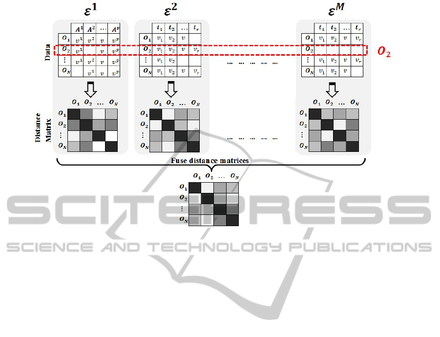
Figure 1: Heterogeneous data representation: The red dashed rectangle shows the data relating to a particular object,O
2
,
whereas the matrices show various elements including a SD element,E
1
, and two TS elements,E
2
and E
M
. The lower part of
the diagram shows the fusion strategy that results from producing a distance matrix for each element and fusing them together
to create a unique distance matrix for all objects.
Attribute to be stored with its corresponding value,
whereas for a TS element the field corresponds to
the time with its corresponding value. An exam-
ple of a patient data recorded in this way may be:
< Pat123,HISData,age,57 >,
< Pat123,HISData,weight,66 >,
< Pat123,HISData,tumourStage,3 >
< Pat123,BloodVitaminD,0,13.2 >
< Pat123,BloodVitaminD,30,13.6 >
< Pat123,BloodVitaminD,65,13.8 >
< Pat123,BloodCalcium,0,39 >
< Pat123,BloodCalcium,30,42 >
< Pat123,BloodCalcium,65,40 >
In this scenario, it is possible to distribute the data us-
ing a distributed file system and it is also possible to
then retrieve the whole dataset for an object or for an
element as required by an algorithm.
4 SIMILARITY MEASURES FOR
HETEROGENEOUS DATA
USING A FUSION APPROACH
Distance measures reflect the degree of (dis)similarity
between objects. From now on we refer to similar-
ity although similarity/dissimilarity are interchange-
able concepts. A variety of measures have been de-
veloped to deal with different data types. Heteroge-
neous data consisting of objects described by differ-
ent data types may require a new way of measuring
distance between objects. In this paper, we are re-
stricting ourselves to two data types: SD and TS data,
however, the approach may be extensible to further
data types. We propose to use a Similarity Matrix Fu-
sion (SMF) approach, as follows: 1. Define a suit-
able data representation to both describe the dataset
and apply suitable distance measures; 2. Calculate
the DMs for each element independently; 3. Consider
how to address data uncertainty; and 4. Fuse the DMs
efficiently into one Fusion Matrix (FM), taking ac-
count of uncertainty.
The main idea of SMF is to create a compre-
hensive view of distances for heterogeneous objects.
SMF computes and fuses DMs obtained from each of
the elements separately, taking advantage of the com-
plementarity in the data. Hence for every pair of ob-
jects, O
i
and O
j
, we begin by calculating entries for
each individual DM corresponding to one of the ele-
ments in the heterogeneous database, E
z
, as follows:
DM
E
z
O
i
,O
j
= dist(O
i
.E
z
,O
j
.E
z
),
where in each case dist represents an appropriate dis-
tance measure for the given data type. When E
z
is
missing in O
i
or O
j
or both the value of DM
E
z
O
i
,O
j
be-
comes null.
Appropriate distance measures are explored in
Section 4.1. The M DMs are later fused into one ma-
KDIR2014-InternationalConferenceonKnowledgeDiscoveryandInformationRetrieval
272

trix, FM, which expresses the distances between het-
erogeneous objects. Along with the process of fusing
DMs, data uncertainty needs to be addressed. Sec-
tion 4.3 describes our suggested solutions. Once we
have a FM representing distances between complex
objects, we can proceed to cluster heterogeneous ob-
jects using standard algorithms. This will be tackled
in further research.
4.1 Construction of DMs for Each
Element
The Standardized Euclidean distance (SEuclidean)
can be employed to measure the similarity for the SD
element because it works efficiently and is well estab-
lished, although other modalities could be explored as
necessary. The SEuclidean distance between SD ele-
ments requires computing the standard deviation vec-
tor S = {s
1
,s
2
,...,s
z
,...,s
p
}, where s
z
is the standard
deviation calculated over the z
th
attribute, A
z
, of the
SD element. SEuclidean between two objects, O
i
and
O
j
, is:
SEuclidean
E
SD
O
i
,O
j
=
p
∑
z=1
(O
i
.E
SD
.A
z
− O
j
.E
SD
.A
z
)
2
/s
z
To measure distance between TSs, we can use a
Dynamic Time Warping (DTW) approach that was
first introduced into the data mining community in
1996 (Berndt and Clifford, 1996). DTW is a non-
linear (elastic) technique that allows similar shapes
to match even if they are out of phase in the time
axis. Ratanamahatana and Keogh (2005) investigated
the ability of DTW to handle sequences of variable
lengths and concluded that reinterpolating sequences
into equal lengths does not produce a statistically sig-
nificant difference to comparing them directly using
DTW. Others (Henniger and Muller, 2007) have ar-
gued that interpolating sequences into equal lengths
is detrimental. We use DTW to assess the TS us-
ing their original lengths. The calculated distances
are normalized and this is achieved by normalizing
through the sum of both series’ lengths. To ex-
plain how to align two TSs using DTW, suppose the
lengths of E
T S
for O
i
and O
j
are r1 and r2 respec-
tively. First, we need to construct an r1 × r2 piece-
wise squared distance matrix. The k
th
element of this
matrix, W
k
, coresponds to the squared distance be-
tween the k
th
pair of values , v
z
and v
l
of TS ele-
ments of O
i
and O
j
respectively which is calculated
as (O
i
.E
T S
.v
z
− O
j
.E
T S
.v
l
)
2
. Then the DTW dis-
tance for E
T S
of O
i
and O
j
is defined by the short-
est path through this matrix. The optimal path can be
found using dynamic programming (Ratanamahatana
and Keogh, 2005) that minimises the warping cost:
DTW
E
T S
O
i
,O
j
= min
(
s
K
∑
k=1
W
k
All the computed distances in the M DMs need
to be normalized to lie in the range [0 − 1] since this
is essential in handling data uncertainty which is dis-
cussed in Section 4.3. Principally, our method is gen-
eral and can be extended to other data types by using
relevant distance measure, e.g. cosine similarity for
text elements or Earth Mover’s Distance for image el-
ements.
4.2 Computing the Fusion Matrix
Fusion of the M DMs for each element can be
achieved using a weighted average approach. Weights
are used to allow emphasis on those elements that
may have more influence on discriminating the ob-
jects. When all elements are to contribute equally to
the calculations, all weights can be set to 1. The fused
matrix representing the distance between two objects,
FM
O
i
,O
j
, can be defined as:
FM
O
i
,O
j
=
M
∑
z=1
w
z
× DM
E
z
O
i
,O
j
M
∑
z=1
w
z
∀i, j ∈ {1,2...N}. w
z
is the weight given to the z
th
el-
ement.
4.3 How to Handle Uncertainty
Uncertainty is inseparably associated with learning
from data. Cormode and McGregor (2008) reported
that combining data values, can be considered as a
source of uncertainty. Thus in our research the pro-
cess of measuring similarity can be affected by un-
certainty in a number of ways. First, we may be
comparing incomplete objects. Assessing similar-
ity for incomplete objects produces a null value in
DM
E
z
O
i
,O
j
when either O
i
and/or O
j
are missing for the
z
th
element. Secondly, a lack of coincidence (or dis-
cordance) in assessing the distance between objects
when using different elements may also introduce un-
certainty in the FM. For instance, O
i
and O
j
may
be considered as similar objects in some of the pre-
computed DMs but not in others, making the overall
similarity of the objects uncertain.
We propose a description for both types of uncer-
tainty as follows. For each pair of objects,O
i
and O
j
,
AFusionApproachtoComputingDistanceforHeterogeneousData
273

we compute the uncertainty associated with the FM
arising from missing information, UFM, as follows:
UFM
O
i
,O
j
=
1
M
M
∑
z=1
(
1, DM
E
z
O
i
,O
j
6= null
0, otherwise
With regards to the disagreement between DMs judg-
ments, we compute the uncertainty associated with
the FM, DFM, for each pair of objects,O
i
and O
j
, as
follows:
DFM
O
i
,O
j
=
1
M
M
∑
z=1
(DM
E
z
O
i
,O
j
− DM
O
i
,O
j
)
2
!
1
2
,
where,
DM
O
i
,O
j
=
1
M
M
∑
z=1
DM
E
z
O
i
,O
j
In other words, UFM, calculates the proportion of
missing distance values in the DMs associated with
all elements for objects O
i
and O
j
, while DFM, cal-
culates the standard deviation of distance values in
the DMs associated with all elements for objects O
i
and O
j
. We now have two expressions of uncertainty,
UFM and DFM, associated with each value of the fu-
sion matrix, FM. Those values may be used separately
to filter data or combined together. We may wish to
use UFM and DFM individually to filter out uncer-
tain values according to different criteria, or we may
wish to report both values together, for example by
calculating the average of both measures as the uncer-
tainty associated with a given value of FM. To filter
out values we can set thresholds for each calculation
individually, i.e., ignoring cases where UFM ≥ φ
1
or
DFM ≥ φ
2
.
5 THE EXPERIMENTAL WORK
5.1 Dataset Used
A real dataset was used for the experiments. It ini-
tially included descriptions of a total of 1,904 patients
diagnosed with prostate cancer at the Norwich and
Norfolk University Hospital (NNUH), UK. It was cre-
ated by Bettencourt-Silva et al. (2011) by integrating
data from nine different hospital information systems.
Each patient’s data is represented by 26 attributes that
form the SD part of the data. They describe demo-
graphics (e.g. age, death indicator) and other disease
states (e.g. Gleason score, tumor staging). In addi-
tion, 23 different blood test results are recorded as TS
(e.g. Vitamin D, MCV, Urea). For the TS, time is
considered as 0 at time of diagnosis and then reported
as number of days from diagnosis. Data on all TSs
before diagnosis was discarded and z-normalization
was conducted on all values in the TSs before calcu-
lating distances. This was done for each E
TS
element
separately, i.e. each TS then has values that have been
normalised across all patients for that particular E
TS
to achieve mean equal to 0 and unit variance. Also,
we cleaned the data by discarding blood tests where
there was mostly missing data for all patients, and re-
moved patients which appeared to hold invalid val-
ues for some attributes, etc. At the end of this stage,
we still had 1,598 patient objects with SD for 26 at-
tributes and 22 distinct TSs.
5.2 A Worked Example
To understand how our approach applies to data, we
select a small sample of 16 patients that represent the
following scenarios:
S1 4 patients, O
1
: O
4
, that are described as complete
heterogeneous objects, with 22 TSs and SD ele-
ment with 26 recorded values. Manual examina-
tion of the raw data indicated they are very similar
(but not identical) in all of their elements. Thus,
we are certain that they are similar.
S2 4 patients, O
5
: O
8
, that are described as complete
heterogeneous objects, with 22 TSs and SD el-
ement with 26 recorded values. Manual exam-
ination of the raw data shows they are dissimi-
lar, and all their DMs reported concordant large
values (associated with dissimilarity). Thus, we
are certain that they are dissimilar according to all
their elements.
S3 The same 4 patients in S1 are used with some of
their elements discarded to create uncertainty, O
9
:
O
12
. They all hold a complete SD element but
are described by different number of TSs as we
have removed some. The no. of present TSs are
O
9
=14, O
10
=16, O
11
=13 and O
12
=15. Thus, they
are similar but we are uncertain as the objects are
incomplete.
S4 O
13
: O
16
, the same 4 patients in S2 but with some
added noise to the raw data so that they reported
large but divergent similarity according to the dif-
ferent DMs. Also we discarded some of the TSs
so the no. of TSs present are: O
13
=15, O
14
=16,
O
15
=17 and O
17
=12. Thus, they are dissimilar but
we are uncertain as disagreement and objects’ in-
completeness are present.
Note that in the process of removing TSs, we some-
times deleted the same TS element, E
TSi
, from two
objects and other times we discarded different TSs,
E
TSi
and E
TSj
, in order to test both cases.
KDIR2014-InternationalConferenceonKnowledgeDiscoveryandInformationRetrieval
274
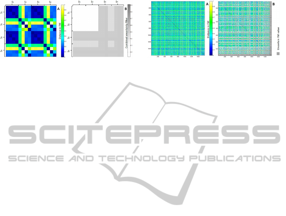
Figure 2: FM for the data sample (A, to the left) and its
combined uncertainty filter (B, to the right). The uncer-
tainty filter reports the average of UFM and DFM. In A,
dark blue reflects strong similarity (FM≤0.1) and then it
scales through green until it reaches bright yellow to reflect
dissimilarity (FM=0.9). In B, the scales of grey colour re-
port uncertainty, the darker the colour the higher the level of
uncertainty. The white area in B supports the FM calcula-
tions for S
1
and S
2
cases with combined uncertainty values
≤ 0.05. The other calculations are subject to varying levels
of uncertainty.
Patients in the sample were compared to each
other following our SMF approach. Objects in S1 re-
ported similarity values in the FM < 0.2 while the
FM similarities for patients in S2 were > 0.7. Both
had all associated variance values, DFM, ≤ 0.1 and
incompleteness values, UFM, equal to 0. Patients in
S3 reported similarity values in FM < 0.2 with vari-
ances reported in DFM ≤ 0.2 and incompleteness val-
ues in UFM > 0.4. Patients in S4 reported similarity
values > 0.7 in FM with variances in DFM > 0.2 and
incompleteness in UFM > 0.4.
Figure 2 provides a visulisation of our results for
the small sample of data whereas Figure 3 gives the
FM visualisation for the entire patient dataset. In Fig-
ure 2 the UFM and DFM are used to report uncer-
tainty in the right hand heatmap (coloured in grey).
We can see in the heatmap on the right that patients
from S1 and S2 are similar/dissimilar respectively but
in both cases the similarity reported in the FM is cer-
tain according to the companion uncertainty heatmap.
On the other hand, patients in S3 are still similar (as
they related to S1 patients) but report higher levels of
uncertainty, whereas the S4 patients are both dissimi-
lar (as they relate to S2) and uncertain.
In Figure3 the heatmap on (A) represents FM sim-
ilarities for the whole dataset and in (B) the same FM
is presented but this time using uncertainty thresholds.
In this case, the companion UFM and DFM values are
used to highlight patients (coloured in grey) where
uncertainty is above predetermined thresholds. Any
value in the FM associated with a UFM value < 0.4%
or a DFM > 0.1 is coloured in grey.
Figure 3: FMs for the cancer heterogeneous dataset before
(A) and after (B) using a combined uncertainty filter that
sets the thresholds for UFM=0.4 and DFM=0.1. In A, dark
blue reflects strong similarity (FM≤0.09) and then it scales
through green until it reaches bright yellow to reflect dis-
similarity (FM=0.9. The same applies in B, in addition to
having the grey colour to represent all patients that report
uncertain distance values in FM due to exceeding one or
both of the determined thresholds.
6 CONCLUSIONS
We have defined heterogeneous datasets as those de-
scribing complex objects comprising of several data
categories including structured data, images, free text,
time series and others. The analysis of such complex
data is one of the biggest challenges facing pattern
analysis tasks, yet few efforts have been devoted to
reaching a mature understanding of this problem. In
this research we propose an intermediary fusion ap-
proach, SFM, which produces a matrix of distances
for complex objects enabling the application of stan-
dard clustering algorithms. SMF aggregates partial
distances that we compute separately on each data
element. We enhance our approach by considering
uncertainty and providing separate measures of the
uncertainty involved both with missing elements and
with diverging distance measures.
We have proposed a very general approach which
can be applied to any problem where objects are de-
scribed by different data types corresponding to dif-
ferent elements or views of the same object. Provid-
ing suitable measures of distance can be found and
used to produce a normalised DM for each element,
such DMs can be fused with others using our ap-
proach. This intermediate fusion allows for the appli-
cation of standard clustering algorithms on the fused
distances. However, clustering results may be en-
hanced by modifying the clustering algorithm to take
accoung of the information contained in the compan-
ion matrices that describe uncertainty.
We provide some preliminary experimental appli-
cation to a real dataset of prostate cancer patients de-
fined by both standard data and a number of TSs rep-
resenting blood test results. We show a worked exam-
ple of distance and uncertainty calculations and show
AFusionApproachtoComputingDistanceforHeterogeneousData
275

how the values may be visualised via heatmaps.
Further research would be required to fully evalu-
ate our approach and provide results including those
generated by clustering data using our fused dis-
tances. We will also need to compare our interme-
diary fusion approach with a late fusion approach us-
ing an ensemble clustering algorithm to perform the
clustering of complex objects.
REFERENCES
Berndt, D. J. and Clifford, J. (1996). Finding patterns in
time series: A dynamic programming approach. In
Fayyad, U. M., Piatetsky-Shapiro, G., Smyth, P., and
Uthurusamy, R., editors, Advances in Knowledge Dis-
covery and Data Mining, pages 229–248. American
Association for Artificial Intelligence, Menlo Park,
CA, USA.
Bettencourt-Silva, J., Iglesia, B. D. L., Donell, S., and
Rayward-Smith, V. (2011). On creating a patient-
centric database from multiple hospital information
systems in a national health service secondary care
setting. Methods of Information in Medicine, pages
6730–6737.
Bostr
¨
om, H., Andler, S. F., Brohede, M., Johansson, R.,
Karlsson, A., van Laere, J., Niklasson, L., Nilsson,
M., Persson, A., and Ziemke, T. (2007). On the defini-
tion of information fusion as a field of research. Tech-
nical report, Institutionen f
¨
or kommunikation och in-
formation.
Cormode, G. and McGregor, A. (2008). Approximation al-
gorithms for clustering uncertain data. In Proceed-
ings of the Twenty-seventh ACM SIGMOD-SIGACT-
SIGART Symposium on Principles of Database Sys-
tems, PODS ’08, pages 191–200, New York, NY,
USA. ACM.
Dimitriadou, E., Weingessel, A., and Hornik, K. (2002). A
combination scheme for fuzzy clustering. In Pal, N.
and Sugeno, M., editors, Advances in Soft Computing
AFSS 2002, volume 2275 of Lecture Notes in Com-
puter Science, pages 332–338. Springer Berlin Hei-
delberg.
Evrim, Rasmussen, M. A., Savorani, F., Ns, T., and Bro,
R. (2013). Understanding data fusion within the
framework of coupled matrix and tensor factoriza-
tions. Chemometrics and Intelligent Laboratory Sys-
tems, 129(9):53–63.
Goh, C. (1996). Representing and reasoning about semantic
conflicts. In In Heterogeneous Information System,
PhD Thesis, MIT.
Greene, D. and Cunningham, P. (2009). A matrix factoriza-
tion approach for integrating multiple data views. In
Buntine, W., Grobelnik, M., Mladeni, D., and Shawe-
Taylor, J., editors, Machine Learning and Knowl-
edge Discovery in Databases, volume 5781 of Lecture
Notes in Computer Science, pages 423–438. Springer
Berlin Heidelberg.
Henniger, O. and Muller, S. (2007). Effects of time normal-
ization on the accuracy of dynamic time warping. In
Biometrics: Theory, Applications, and Systems, 2007.
BTAS 2007. First IEEE International Conference on,
pages 1–6.
Jain, A. K., Murty, M. N., and Flynn, P. J. (1999). Data
clustering: A review. ACM Comput. Surv., 31(3):264–
323.
Kim, W. and Seo, J. (1991). Classifying schematic and data
heterogeneity in multidatabase systems. Computer,
24(12):12–18.
Laney, D. (2001). 3D data management: Controlling data
volume, velocity, and variety. Technical report, META
Group.
Long, B., Zhang, Z., Wu, X., and Yu, P. S. (2006). Spec-
tral clustering for multi-type relational data. In ICML,
pages 585–592.
Ma, H., Yang, H., Lyu, M. R., and King, I. (2008).
Sorec: Social recommendation using probabilistic
matrix factorization. In Proceedings of the 17th ACM
Conference on Information and Knowledge Manage-
ment, CIKM ’08, pages 931–940, New York, NY,
USA. ACM.
Maragos, P., Gros, P., Katsamanis, A., and Papandreou,
G. (2008). Cross-modal integration for performance
improving in multimedia: A review. In Maragos,
P., Potamianos, A., and Gros, P., editors, Multimodal
Processing and Interaction, volume 33 of Multimedia
Systems and Applications, pages 1–46. Springer US.
Pavlidis, P., Cai, J., Weston, J., and Noble, W. S. (2002).
Learning gene functional classifications from multi-
ple data types. Journal of Computational Biology,
9(2):401–411.
Ratanamahatana, C. A. and Keogh, E. (2005). Three myths
about dynamic time warping data mining. Proceed-
ings of SIAM International Conference on Data Min-
ing (SDM05), pages 506–510.
Skillicorn, D. B. (2007). Understanding Complex Datasets:
Data Mining with Matrix Decompositions. Chapman
and Hall/CRC, Taylor and Francis Group.
Strehl, A. and Ghosh, J. (2003). Cluster ensembles — a
knowledge reuse framework for combining multiple
partitions. J. Mach. Learn. Res., 3:583–617.
ˇ
Zitnik, M. and Zupan, B. (2014). Matrix factorization-based
data fusion for gene function prediction in baker’s
yeast and slime mold. Systems Biomedicine, 2:1–7.
van Vliet, M. H., Horlings, H. M., van de Vijver, M. J.,
Reinders, M. J. T., and Wessels, L. F. A. (2012). In-
tegration of clinical and gene expression data has a
synergetic effect on predicting breast cancer outcome.
PLoS ONE, 7(7):e40358.
Yu, S., Falck, T., Daemen, A., Tranchevent, L.-C., Suykens,
J., De Moor, B., and Moreau, Y. (2010). L2-norm mul-
tiple kernel learning and its application to biomedical
data fusion. BMC Bioinformatics, 11(1).
Zeng, H.-J., Chen, Z., and Ma, W.-Y. (2002). A unified
framework for clustering heterogeneous web objects.
In Web Information Systems Engineering, 2002. WISE
2002. Proceedings of the Third International Confer-
ence, pages 161–170.
KDIR2014-InternationalConferenceonKnowledgeDiscoveryandInformationRetrieval
276
