
Particle Swarms with Dynamic Topologies and Conservation of
Function Evaluations
Carlos M. Fernandes
1
, Juan L. J. Laredo
2
, Juan Julian Merelo
3
, Carlos Cotta
4
and Agostinho Rosa
1
1
LARSyS: Laboratory for Robotics and Systems in Engineering and Science, University of Lisbon,
Av. Rovisco Pais, 1, Lisbon, Portugal
2
Faculty of Sciences, Technology and Communications, University of Luxembourg,
6, rue Richard Coudenhove-Kalergi, L-1359, Luxembourg, Luxembourg
3
Departamento de Arquitectura y Tecnología de Computadores, University of Granada,
C/ Daniel Saucedo Aranda, s/n, 18071, Granada, Spain
4
Lenguages y Ciencias de la Computacion, Universidad de Malaga, ETSI Informática (3.2.49),
Universidad de Málaga, Campus de Teatinos, 29071, Malaga, Spain
Keywords: Particle Swarm Optimization, Population Structure, Dynamic Topologies, Swarm Intelligence.
Abstract: This paper proposes a general framework for structuring dynamic Particle Swarm populations and uses a
conservation of function evaluations strategy to increase the convergence speed. The population structure is
constructed by placing the particles on a 2-dimensional grid of nodes, where they interact and move
according to simple rules. During the running time of the algorithm, the von Neumann neighborhood is used
to decide which particles influence each other when updating their velocity and position. Each particle is
updated in each time-step but they are evaluated only if there are other particles in their neighborhood. A set
of experiments demonstrates that the dynamics imposed by the structure provides a more consistent and
stable behavior throughout the test set when compared to standard topologies, while the conservation of
evaluations significantly reduces the convergence speed of the algorithm. Furthermore, the working
mechanisms of the proposed structure are very simple and, except for the size of the grid, they do not
require parameters and tuning.
1 INTRODUCTION
Kennedy and Eberhart (1995) proposed the Particle
Swarm Optimization (PSO) algorithm for binary and
real-valued function optimization, a method inspired
by the swarming and social behavior of bird flocks
and fish schools. Since then, PSO has been applied
with success to a wide range of problems but the
proper balance between exploration (global search)
and exploitation (local search) is still an open
problem that motives several lines research on the
various mechanisms that control the algorithm’s
performance.
Population topology is one of PSO’s components
that affect the balance between exploration and
exploitation and the convergence speed and
accuracy of the algorithm. In the context of particle
swarms, topology is the structure that defines the
connections between the particles and consequently
the flow of information through the population. The
reason why particles are interconnected is the core
of the algorithm: the particles communicate so that
they acquire information on the regions explored by
other particles. In fact, it has been claimed that the
uniqueness of the PSO algorithm lies in the
interactions of the particles (Kennedy and Mendes,
2002). The population can be structured on any
possible topology, from sparse to dense (or even
fully connected) graphs), with different degrees of
connectivity and clustering. The classical and most
used population structures are the lbest (which
connects the individuals to a local neighborhood)
and the gbest (in which each particle is connected to
every other individual). These topologies are well-
studied and the major conclusions are that gbest is
fast but is frequently trapped in local optima, while
lbest is slower but converges more often to the
neighborhood of the global optima.
Since the first experiments on lbest and gbest
structures, researchers have tried to design networks
that hold the best traits given by each structure
86
Fernandes C., Laredo J., Merelo J., Cotta C. and Rosa A..
Particle Swarms with Dynamic Topologies and Conservation of Function Evaluations.
DOI: 10.5220/0005087900860094
In Proceedings of the International Conference on Evolutionary Computation Theory and Applications (ECTA-2014), pages 86-94
ISBN: 978-989-758-052-9
Copyright
c
2014 SCITEPRESS (Science and Technology Publications, Lda.)

(Parsopoulos and Vrahatis, 2004). Some studies also
try to understand what makes a good structure: for
instance, Kennedy and Mendes (2002) investigate
several types of topologies and recommend the use
of a lattice with von Neumann neighborhood (which
results in a connectivity degree between that of lbest
and gbest).
Recently, dynamic structures have been tested in
order to improve the algorithm’s adaptability to
different fitness landscapes and overcome the
rigidity of static structures, like in (Liang et al.,
2006). Fernandes et al. (2003) try a different
approach and propose a dynamic and partially
connected von Neumann structure with Brownian
motion. This paper uses this model but introduces a
strategy for the conservation of function evaluations
(Majercik, 2013) with the aim of taking advantage of
the underlying structure and reduce convergence
speed. Furthermore, a formal description of the
dynamic network is given here, opening the way for
more sophisticated dynamics.
In the proposed topology, particles are placed in a
2-dimensional m-nodes grid where . Every
time-step, each individual checks its von Neumann
neighborhood and, as in the standard PSO, updates
its velocity and position using the information given
by the neighbors. However, while the connectivity
degree (number of numbers, considering the particle
itself) of the von Neumann topology is 5, the
degree of the proposed topology is variable: 5.
Furthermore, the structure is dynamic: in each time-
step, every particle updates its position on the grid
(which is a different concept from the position of the
particle on the fitness landscape) according to a pre-
defined rule that selects the destination node. The
movement rule, which is implemented locally and
without any knowledge on the global state of the
system, can be based on stigmergy (Grassé, 1959) or
Brownian motion.
As stated above, the connectivity degree of each
particle in each time-step is variable and lies in the
range 15. Depending on the size of the grid,
there are, in each time-step, a number of particles
with 1. These particles without neighbors
(except the particle itself) do not learn from any
local neighborhood at that specific iteration.
Therefore, it is expected that they continue to follow
their previous trajectory in the fitness landscape.
Taking into account these premises, the algorithm
proposed in this study does evaluate the position of
the particles when 1. Regardless of the loss of
informant intrinsic to a conservation of evaluations
policy, we hypothesize that the strategy is
particularly suited for the proposed dynamic
topology (in which the particles are sometimes
isolated from the flow of information) and the
number of function evaluations required for meeting
the stop criteria can be significantly reduced.
Furthermore, it is the structure of the population and
the position of the particles at a specific time-step
that decides the application of the conservation rule
and not any extra parameter or pre-defined decision
rule.
A classical PSO experimental setup is used for the
tests and the results demonstrate that the proposed
algorithm consistently improves the speed of
convergence of the standard von Neumann structure
without degrading the quality of solutions. The
experiments also demonstrate that the introduction
of the conservation strategy reduces significantly the
convergence speed without affecting the quality of
the final solutions.
The remaining of the paper is organized as follows.
Section 2 describes PSO and gives an overview on
population structures for PSOs. Section 3 gives a
formal description of the proposed structure. Section
4 describes the experiments and discusses the results
and, finally, Section 5 concludes the paper and
outlines future research.
2 BACKGROUND REVIEW
PSO is described by a simple set of equations that
define the velocity and position of each particle. The
position of the i-th particle is given by
,
,
,
,…
,
), where is the dimension of the
search space. The velocity is given by
,
,
,
,…
,
). The particles are evaluated with a
fitness function
and then their positions and
velocities are updated by:
,
,
1
,
,
1
,
,
1
(1)
,
,
1
,
(2)
were
is the best solution found so far by particle
and
is the best solution found so far by the
neighborhood. Parameters
and
are random
numbers uniformly distributed in the range 0,1] and
and
are acceleration coefficients that tune the
relative influence of each term of the formula. The
first term is known as the cognitive part, since it
relies on the particle’s own experience. The last term
ParticleSwarmswithDynamicTopologiesandConservationofFunctionEvaluations
87

is the social part, since it describes the influence of
the community in the trajectory of the particle.
In order to prevent particles from stepping out of the
limits of the search space, the positions
,
are
limited by constants that, in general, correspond to
the domain of the problem:
,
∊
,
. Velocity may also be
limited within a range in order to prevent the
explosion of the velocity vector:
,
∊
,
.
For achieving a better balancing between local and
global search, Shi an Eberhart (1998) added the
inertia weight as a multiplying factor of the first
term of equation 1. This paper uses PSOs with
inertia weight.
The neighborhood of the particle defines the value
of
and is a key factor in the performance of PSO.
Most of the PSOs use one of two simple sociometric
principles for defining the neighborhood network.
One connects all the members of the swarm to one
another, and it is called gbest, were g stands for
global. The degree of connectivity of gbest is ,
where is the number of particles. Since all the
particles are connected to every other and
information spreads easily through the network, the
gbest topology is known to converge fast but
unreliably (it often converges to local optima).
The other standard configuration, called lbest (where
l stands for local), creates a neighborhood that
comprises the particle itself and its nearest
neighbors. The most common lbest topology is the
ring structure, in which the particles are arranged in
a ring structure (resulting in a degree of connectivity
3, including the particle). The lbest converges
slower than the gbest structure because information
spreads slower through the network but for the same
reason it is less prone to converge prematurely to
local optima. In-between the ring structure with
3 and the gbest with there are several
types of structure, each one with its advantages on a
certain type of fitness landscapes. Choosing a proper
structure depends on the target problem and also on
the objectives or tolerance of the optimization
process.
Kennedy and Mendes (2002) published an
exhaustive study on population structures for PSOs.
They tested several types of structures, including the
lbest, gbest and von Neumann configuration with
radius 1 (also kown as 5 neighborhood). They also
tested populations arranged in randomly generated
graphs. The authors conclude that when the
configurations are ranked by the performance the
structures with k = 5 (like the 5) perform better,
but when ranked according to the number of
iterations needed to meet the criteria, configurations
with higher degree of connectivity perform better.
These results are consistent with the premise that
low connectivity favors robustness, while higher
connectivity favors convergence speed (at the
expense of reliability). Amongst the large set of
graphs tested in (Kennedy and Mendes, 2002), the
Von Neumann with radius 1 configuration
performed more consistently and the authors
recommend its use.
Alternative topologies that combine standard
structures’ characteristics or introduce some kind of
dynamics in the connections have been also
proposed. Parsopoulos and Vrahatis (2004) describe
the unified PSO (UPSO), which combines the gbest
and lbest configurations. Equation 1 is modified in
order to include a term with
and a term with
and a parameter balances the weight of each term.
The authors argue that the proposed scheme exploits
the good properties of gbest and lbest. Peram et al.
(2003) proposed the fitness–distance-ratio-based
PSO (FDR-PSO), which defines the “neighborhood”
of a particle as its closest particles in the
population (measured by the Euclidean distance). A
selective scheme is also included: the particle selects
nearby particles that have also visited a position of
higher fitness. The algorithm is compared to a
standard PSO and the authors claim that FDR-PSO
performs better on several test functions. However,
the FDR-PSO is compared only to a gbest
configuration, which is known to converge
frequently to local optima in the majority of the
functions of the test set. More recently, a
comprehensive-learning PSO (CLPSO) was
proposed (Liang et al. 2006). Its learning strategy
abandons the global best information and introduces
a complex and dynamic scheme that uses all other
particles’ past best information. CLPSO can
significantly improve the performance of the
original PSO on multimodal problems. Finally,
Hseigh et al. (2009) use a PSO with varying swarm
size and solution-sharing that, like in (Liang et al.
2006), uses the past best information from every
particle.
A different approach is given in (Fernandes et al.,
2013). The authors describe a structure that is based
on a grid of nodes (with ) on which the
particles move and interact. The von Neumann
neighborhood is checked for chosing the informants
of the cognitive part of equation 1. Since , the
number of neighbors lies in the range 15 and
ECTA2014-InternationalConferenceonEvolutionaryComputationTheoryandApplications
88

the distribution of the particles on the grid at a given
time-step defines the PSO structure at that precise
iteration. The results demonstrate that the proposed
structure performs consistently throughout the test
set, improving the performance of other topologies
in the majority of the scenarios and under different
performance evaluation criteria. Furthermore, the
structure is very simple and only the grid size needs
to be set before the run (the authors suggest 1:2 ratio
between the swarm size and the number of nodes).
However, the structure itself and the distribution of
the particles on the grid suggest that there is still
room for improvement, namely of convergence
speed, which is a critical aspect when optimizing
real-world functions.
In the proposed structure, a particle, at a given time-
step, may have no neighbors except itself. The
isolated particles will continue to follow its previous
trajectory, based on their current information, until
they find another particle in the neighborhood.
Therefore, we intend to investigate if the loss of
information caused by not evaluating these particles
is overcome by the payoff in the convergence speed.
Common ways of addressing the computational cost
of evaluating solutions in hard real-world problems
are function approximation (Landa-Becerra et al.,
2008), fitness inheritance (Reyes-Sierra and Coello
Coello, 2007) and conservation of evaluations
(Majercik, 2013). Due to the underlying structure of
the proposed algorithm, we have tested a
conservation policy similar to the GREEN-PSO
proposed by Majercik (2013). However, in our
algorithm the decision on evaluating or not is made
by the position of the particle in the grid (isolated
particles are not evaluated) while in the GREEN-
PSO the decision is probabilistic and the likelihood
of conserving a solution is controlled by a
parameter.
The following section gives a formal description of
the proposed network and presents the transition
rules that define the model for dynamic population
structures.
3 PARTIALLY CONNECTED
STRUCTURES
Let us consider a rectangular grid of size
, where is the size of the population of any
population-based metaheuristics or model. Each
node
of the grid is a tuple
〈
,
〉
, where
∈
1,…,
∪
•
and
∈
∪
•
for
some domain . The value
indicates the index
of the individual that occupies the position
〈
,
〉
in
the grid. If
• then the corresponding position
is empty. However, that same position may still have
information, namely a mark (or clue)
. If
= •
then the position is empty and unmarked. Please
note that when , the topology is a static 2-
dimensional lattice and when and
the topology is the standard square grid graph.
In the case of a PSO, the marks are placed by
particles that occupied that position in the past and
they consist of information about those particles,
like their fitness
or position in the fitness
landscape, as well as a time stamp
that indicates
the iteration in which the mark was placed. The
marks have a lifespan of iterations, after which
they are deleted.
Initially,
•,• for all
〈
,
〉
. Then, the
particles are placed randomly on the grid (only one
particle per node). Afterwards, all particles are
subject to a movement phase (or grid position
update), followed by a PSO phase. The process
(position update and PSO phase) repeats until a stop
criterion is met.
The PSO phase is the standard iteration of a PSO,
comprising position and velocity update. The only
difference to a static structure is that in this case a
particle may find empty nodes in its neighborhood.
In the position update phase, each individual moves
to an adjacent empty node. Adjacency is defined by
the Moore neighborhood of radius , so an
individual at
〈
,
〉
can move to an empty
node
〈
,
〉
for which
〈
,
〉
,
〈
,
〉
. If
empty positions are unavailable, the individual stays
in the same node. Otherwise, it picks a neighboring
empty node according to the marks on them. If there
are no marks, the destination is chosen randomly
amongst the free nodes.
With this framework, there are two possibilities for
the position update phase: stimergic, whereby the
individual looks for a mark that is similar to itself;
and Brownian, whereby the individual selects an
empty neighbor regardless of the marks. For the first
option, let
〈
,
〉
〈
,
〉
,…,
〈
,
〉
be
the collection of empty neighboring nodes and let
be the individual to move. Then, the individual
attempts to move to a node whose mark is as close
as possible to its own corresponding trait (fitness or
position in the fitness landscape, for instance) or to
an adjacent cell picked at random if there are no
marks in the neighborhood. In the alternative
Brownian policy, the individual moves to an
ParticleSwarmswithDynamicTopologiesandConservationofFunctionEvaluations
89

adjacent empty position picked at random. In either
case, the process is repeated for the whole
population.
For this paper, the investigation is restricted to the
Brownian structure. The algorithm is referred in the
remaining of the paper has PSO-B, followed by the
grid size . An extension of the PSO-B is also
proposed by introducing a conservation of function
evaluations (cfe) strategy. If at a given time-step a
particle has no neighbors, then the particle is
updated but its position is not evaluated. This
version of the algorithm is referred to as PSO-Bcfe.
The following section describes the results attained
by the PSOs with dynamic structure and Brownian
movement, with and without conservation of
function evaluations and compares them to the
standard topologies.
4 EXPERIMENTS AND RESULTS
This section describes the experiments conducted for
evaluating the performance of the proposed stru-
cture. The algorithm is first compared to the version
without conservation of function evaluations.
Table 1: Benchmarks for the experiments. Dynamic range,
initialization range and stop criteria.
function
mathematical
representation
Rangeof
search/
Rangeof
initialization
stop
Sphere
f
1
100,100
(50,100
0.01
Rosenbrock
f
2
100
1
100,100
15,30
100
Rastrigin
f
3
10cos
2
10
10,10
2.56,5.12
100
Griewank
f
4
1
1
4000
cos
√
600,600
300,600
0.05
Schaffer
f5
0.5
sin
0.5
1.00.001
100,100
15,30
0.00001
Table 2: PSO-B and PSO-Bcfe. Best fitness values
averaged over 50 runs.
f
1
f
2
f
3
f
4
f
5
PSO-B
8×8
2.71e‐40 7.98e+00 6.57e+01 7.43e‐03 1.17e‐03
±4.21e‐40 ±1.11e+01 ±1.78e+01±9.02e‐03 ±3.19E‐03
PSO-Bcfe
8×8
3.20e‐40 1.12e+01 6.29e+01 7.44e‐03 1.94e‐04
±8.44e‐40 ±2.02e+01 ±1.35e+01±7.96e‐03±1.37E‐03
PSO-B
10×10
8.74e‐38 1.25e+01 6.23e+01 7.73e‐03 0.00e+00
±1.29e‐37 ±2.07e+01 ±1.88e+01±9.50e‐03±0.00E+00
PSO-Bcfe
10×10
2.43e‐39 1.09e+01 6.16e+01 5.61e‐03 0.00e+00
±4.38e‐39 ±1.67e+01 ±1.60e+01±7.47e‐03±0.00E+00
PSO-B
15×15
3.47e‐33 1.53e+01 6.05e+01 3.79e‐03 3.89e‐04
±4.31e‐33 ±2.65e+01 ±1.45e+01±6.22e‐03±1.92E‐03
PSO-Bcfe
15×15
2.47e‐45 1.31 e+01 6.62e+01 6.45e‐03 0.00e+00
±4.21e‐45 ±2.42e+01 ±2.05e+01±9.90e‐03±0.00E+00
Then, the topology with Brownian motion and
conservation of evaluations is compared to the lbest,
gbest, and standard square von Neumann topologies.
An experimental setup was constructed with five
benchmark unimodal and multimodal functions that
are commonly used for investigating the
performance of PSO − see (Kennedy and Mendes,
2002) and (Trelea, 2003) for instance). The
functions are described in Table 1. The optimum
(minimum) of all functions is located in the origin
with fitness 0. The dimension of the search space is
set to 30 (except Schaffer, with 2). In
order to set a square grid graph for the standard von
Neumann topology, the population size is set to 49
(which is within the typical range of PSO’s swarm
size). The acceleration coefficients were set to 1.494
and the inertia weight is 0.729, as in (Trelea, 2003).
is defined as usual by the domain’s upper
limit and . A total of 50 runs for
each experiment are conducted. Asymmetrical
initialization is used (the initialization range for each
function is given in Table 1).
Two experiments were conducted. Firstly, the
algorithms were run for a limited amount of function
evaluations (147000 for
and
, 49000 for
,
and
) and the fitness of the best solution found was
averaged over the 50 runs. In the second experiment
the algorithms were run for 980000 iterations
(corresponding to 20000 iterations of standard PSO
with 49) or until reaching the stop criterion.
The criteria were taken from (Kennedy and Mendes,
2002) and are given in Table 1. For each function
and each algorithm, the number of function
evaluations required to meet the criterion is recorded
and averaged over the 50 runs. A success measure is
defined as the number of runs in which an algorithm
ECTA2014-InternationalConferenceonEvolutionaryComputationTheoryandApplications
90

attains the fitness value established as the stop
criterion.
Table 3: PSO-B and PSO-Bcfe. Function evaluations
averaged over 50 runs.
f
1
f
2
f
3
f
4
f
5
PSO-B
8×8
21070.98 56472.50 13224.90 19959.66 14369.25
±1023.60
(50)
±49342.60
(50)
±3894.30
(48)
±1408.36
(50)
±20599.03
(46)
PSO-Bcfe
8×8
21157.7 96148.42 13427.12 19968.40 10275.69
±1092.81
(50)
±112675.6
(50)
±2259.73
(50)
±1103.20
(50)
±6952.548
(49)
PSO-B
10×10
22700.72 65769.76 15114.46 21574.70 10741.78
±906.39
(50)
±70232.15
(50)
±3939.74
(48)
±1107.56
(50)
±10658.16
(50)
PSO-Bcfe
10×10
21796.04 57704.16 13953.04 20430.34 11817.06
±832.54
(50)
±71260.77
(50)
±3341.41
(49)
±1176.32
(50)
±15647.63
(50)
PSO-B
15×15
26122.88 74321.24 20408.50 24626.42 11830.83
±950.08
(50)
±83535.59
(50)
±3692.10
(50)
±1406.53
(50)
±11576.37
(48)
PSO-Bcfe
15×15
19600.76 77348.06 16713.59 18734.94 10890.55
±730.62
(50)
±91374.00
(50)
±4387.78
(46)
±1029.26
(50)
±11624.59
(47)
Table 4: PSO-Bcfe and standard topologies. Best fitness
values averaged over 50 runs.
f
1
f
2
f
3
f
4
f
5
PSO
VN
4.26e‐36 1.39e+01 6.40e+01 5.61e‐03 0.00e+00
±1.32e‐35 ±2.39e+01 ±1.59e+01 ±8.78e‐03 ±0.00e+00
PSO
1.20e‐25 1.19e+01 1.11e+02 2.95e‐04 1.94e‐04
±1.30e‐25 ±2.48e+01 ±1.74e+01 ±2.09e‐03 ±1.37e‐03
PSO
3.80e+03 1.19e+01 9.86e+01 3.80e+01 1.36e‐03
±5.67e+03 ±1.50e+01 ±2.84e+01 ±5.80e+01 ±3.41e‐03
PSO-Bcfe
10×10
2.43e‐39 1.09e+01 6.16e+01 5.61e‐03 0.00e+00
±4.38e‐39 ±1.67e+01 ±1.60e+01 ±7.47e‐03 ±0.00E+00
Table 2 shows the average fitness values attained by
PSO-B and PSO-Bcfe with different grid sizes.
Table 3 shows the average number of function
evaluations required to meet the stop criteria as well
as the number of successful runs. The performance
according to the fitness values is very similar with
no significant differences between the algorithm in
every function except
(PSO-Bcfe is better). When
considering the number of function evaluations (i.e.,
convergence speed), PSO-Bcfe is significantly better
or statistically equivalent in every function. For the
statistical tests comparing two algorithms, non-
parametric Kolmogorov-Smirnov tests (with 0.05
level of significance) have been used.
The results confirm that PSO-Bcfe is able to
improve the convergence speed of PSO-B without
degrading the accuracy of the solutions. The loss of
information that results from conserving evaluations
is clearly overcome by the benefits of reducing the
computational cost per iteration.
In the case of
, PSO-Bcfe also significantly
improves the quality of the solutions, namely with
larger grids. The proposed scheme seems to be
particularly efficient in unimodal landscapes, but
further tests are required in order to confirm this
hypothesis and understand what mechanisms make
PSO-Bcfe so efficient in finding more precise
solutions for the sphere function.
Table 5: PSO-Bcfe and standard topologies. Function
evaluations averaged over 50 runs.
f
1
f
2
f
3
f
4
f
5
PSO
VN
23530.78 72707.18 18424.00 22015.70 17622.36
±954.74
(50)
±92916.33
(50)
±11082.75
(49)
±1304.60
(50)
±16056.6
8
(50)
PSO
32488.96 80547.18 233260.18 30200.66 26263.00
±921.45
(50)
±112067.67
(50)
±281453.62
(17)
±1703.88
1
(50)
±27266.8
6
(49)
PSO
16082.39 56681.24 9602.04 14856.07 13933.09
±2697.41
(33)
±88165.30
(50)
±3599.04
(25)
±2028.12
(27)
±21576.6
3
(43)
PSO-
Bcfe
15×15
21796.04 57704.16 13953.04 20430.34 11817.06
±832.54
(50)
±71260.77
(50)
±3341.41
(49)
±1176.32
(50)
±15647.63
(50)
Figure 1: Rank by Holm-Bonferroni test.
Tables 4 and 5 compare the PSO-Bcfe with standard
PSOs: square grid (77) with von Neumann (VN)
neighborhood, lbest with 3 (ring) and gbest.
As expected, gbest is fast but its solutions are clearly
worst than the other algorithms results (except for
, and
) and the success rates are lower than the
average; lbest is fairly accurate when compared to
other strategies but it clearly requires more
evaluations than the other PSOs in order to meet the
ParticleSwarmswithDynamicTopologiesandConservationofFunctionEvaluations
91
same criteria. The standard von Neumann strategy
and the PSO-Bcfe are more consistent throughout
the test set, but PSO-Bcfe is faster is most of the
functions and significantly faster in
,
, and
. In
addition, its solutions for
are significantly better
than the fitness values attained by the PSO with von
Neumann topology. The proposed strategy maintains
or improves the accuracy of the von Neumann
strategy throughout the test set — the consistency of
the von Neumann topology has been reported by
Kennedy and Mendes (2002) —, while increasing
significantly the convergence speed.
A statistical analysis of the algorithms (including
also PSO-B) on the entire test set was conducted.
First, a Friedman test showed that there are no
significant differences in the performance of the
algorithms considering the fitness values criteria.
When taking into account the function evaluations
and success rates the test reveals significant
differences between the algorithms.
After the Friedman test, a Holm-Bonferroni test was
conducted for ranking the algorithms according to
their convergence speed and reliability and detect
significant differences between the algorithms. PSO-
Bcfe ranks first, followed by PSO-B, PSO with von
Neumann topology, PSO with lbest and finally PSO
with gbest (see Figure 1). Considering 0.1,
PSO-Bcfe is significantly better than the von
Neumann, lbest and gbest topologies. Table 6 shows
the results of the Holm test.
Table 6: Holm test results. .
z‐statistic p‐value
⁄
PSO-B
0.800000 0.211855 0.10000
PSO VN
1.700000 0.044565 0.05000
PSO
2.600000 0.004661 0.33333
PSO
2.900000 0.001866 0.02500
The Holm test concludes that although PSO-Bcfe
attains a better average ranking than PSO-B, there
are no significant differences between the
algorithms. Please remember that the grid size
considered in the general comparisons is 10×10. I
f
we consider a 15×15 grid size we see that PSO-Bcfe
is faster in every function and significantly faster in
f_1, f_3 and f_4, while for grids with size 8×8 the
algorithms are statistically equivalent in ever
y
function. In general, the performance of PSO-Bcfe is
improved or preserved when the grid size grows,
while the performance of PSO-B degrades with the
grid size.
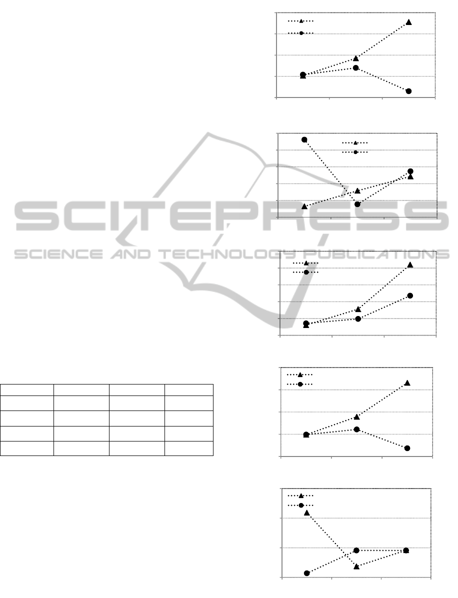
Figure 2: PSO-B and PSO-Bcfe. Function evaluations
required to meet stop criteria when using grids with
different sizes.
19000
21000
23000
25000
27000
8x8 10x10 15x15
functionevaluations
gridsize
spheref1
PSO‐B
PSO‐Bcfe
50000
60000
70000
80000
90000
100000
8x8 10x10 15x15
functionevaluations
gridsize
rosenbrockf2
PSO‐B
PSO‐Bcfe
12000
14000
16000
18000
20000
22000
8x8 10x10 15x15
functionevaluations
gridsize
rastriginf3
PSO‐B
PSO‐Bcfe
18000
20000
22000
24000
26000
8x8 10x10 15x15
functionevaluations
gridsize
griewankf4
VNRAND
G‐PSO
10000
12000
14000
16000
8x8 10x10 15x15
functionevaluations
gridsize
schafferf5
PSO‐B
PSO‐Bcfe
ECTA2014-InternationalConferenceonEvolutionaryComputationTheoryandApplications
92

This behavior may be explained by the fact that in
larger grids the particles are isolated more often and
for longer periods of time. During these periods, the
particles are not using information from the rest of
the swarm. PSO-Bcfe partially overcomes the loss of
communication and information by not evaluating
the particles, thus saving computational resources.
Figure 2 graphically displays the evaluations
required by each version of the algorithm in each
function for different grids. Except for
, PSO-B
number of function evaluations to meet the criteria
increase with the size of the grid, while PSO-Bcfe
scales better, namely in functions
,
and
.
These results show that it is possible to improve
standard PSO’s performance by structuring the
particles on a grid of nodes, let them move
according to simple rules and save computational
resources by letting them follow their current
trajectories without evaluation the new positions.
5 CONCLUSIONS
This paper proposes a general scheme for structuring
dynamic populations for the Particle Swarm
Optimization (PSO) algorithm. The particles are
placed on a grid of nodes where the number of nodes
is larger than the swarm size. The particles move on
the grid according to simple rules and the network of
information is defined by the particle’s position on
the grid and its neighborhood (von Neumann vicinity
is considered here). If isolated (i.e., no neighbors
except itself), a particle is updated but its position is
not evaluated. This strategy results in loss of
information but it decreases the number of
evaluations per generation. The results show that the
payoff in convergence speed overcomes the loss of
information: the number of function evaluations is
reduced in the entire test set, while the accuracy of
the algorithm (i.e., the averaged final fitness) is not
degraded by the conservation of evaluations
strategy.
The proposed algorithm is tested with a Brownian
motion rule and compared to standard static
topologies. Statistical tests and ranking according to
convergence speed and success rates shows that the
dynamic structure with conservation of function
evaluations ranks first and it is significantly better
than the von Neumann, ring and lbest topologies.
Furthermore, the conservation of evaluations
strategy results in a more stable performance when
varying the grid size, while removing this strategy
from the proposed dynamic structure results in a
drop off of the convergence speed when the size of
the grid increases in relation to the swarm size.
The present study is restricted to dynamic structures
based on particles with Brownian motion. However,
a self-organized behavior based on communication
via the grid (stigmergy) can be modeled by the
general framework proposed in this paper. Future
research will be focused on dynamic structures with
stigmergic behavior based on the fitness and position
of the particles.
ACKNOWLEDGEMENTS
The first author wishes to thank FCT, Ministério da
Ciência e Tecnologia, his Research Fellowship
SFRH/ BPD/66876/2009. The work was supported
by FCT PROJECT [PEst-OE/EEI/LA0009/2013],
Spanish Ministry of Science and Innovation projects
TIN2011-28627-C04-02 and TIN2011-28627-C04-
01, Andalusian Regional Government P08-TIC-
03903 and P10-TIC-6083, CEI-BioTIC UGR project
CEI2013-P-14, and UL-EvoPerf project.
REFERENCES
Fernandes, C. M., Laredo, J. L. J., Merelo, J. J., Cotta, C.,
Nogueras, R., Rosa, A.C. 2013. Performance and
Scalability of Particle Swarms with Dynamic and
Partially Connected Grid Topologies. In Proceedings
of the 5th International Joint Conference on
Computational Intelligence IJCCI 2013, pp. 47-55.
Grassé, P.-P. 1959. La reconstrucion du nid et les
coordinations interindividuelles chez bellicositermes et
cubitermes sp. La théorie de la stigmergie: Essai
d’interpretation du comportement des termites
constructeurs, Insectes Sociaux, 6, pp. 41-80.
Hseigh, S.-T., Sun, T.-Y, Liu, C.-C., Tsai, S.-J. 2009.
Efficient Population Utilization Strategy for Particle
Swarm Optimizers. IEEE Transactions on Systems,
Man and Cybernetics—part B, 39(2), 444-456.
Kennedy, J., Eberhart, R. 1995. Particle Swarm
Optimization. In Proceedings of IEEE International
Conference on Neural Networks, Vol.4, 1942–1948.
Kennedy, J., Mendes, R. 2002. Population structure and
particle swarm performance. In Proceedings of the
IEEE World Congress on Evolutionary Computation,
1671–1676.
Landa-Becerra, R., Santana-Quintero, L. V., and Coello
Coello, C. A. 2008. Knowledge incorporation in multi-
objective evolutionary algorithms. In Multi-Objective
Evolutionary Algorithms for Knowledge Discovery
from Databases, pages 23–46.
Liang, J. J., Qin, A. K., Suganthan, P.N., Baskar, S. 2006.
Comprehensive learning particle swarm optimizer for
ParticleSwarmswithDynamicTopologiesandConservationofFunctionEvaluations
93

global optimization of multimodal functions. IEEE
Trans. Evolutionary Computation, 10(3), 281–296.
Majercik, S. 2013. GREEN-PSO: Conserving Function
Evaluations in Particle Swarm Optimization, in
Proceedings of the IJCCI 2013 - International Joint
Conference on Computational Intelligence, pp.160-
167, 2013.
Parsopoulos, K. E., Vrahatis, M. N. 2004. UPSO: A
Unified Particle Swarm Optimization Scheme, Lecture
Series on Computer and Computational Sciences, Vol.
1, Proceedings of the International Conference of
"Computational Methods in Sciences and
Engineering" (ICCMSE 2004), 868-87
Peram, T., Veeramachaneni, K., Mohan, C.K. 2003.
Fitness-distance-ratio based particle swarm
optimization. In Proc. Swarm Intelligence Symposium
SIS’03, IEEE, pp. 174–181.
Reyes-Sierra, M. and Coello Coello, C. A. (2007). A study
of techniques to improve the efficiency of a
multiobjective particle swarm optimizer. In Studies in
Computational Intelligence (51), Evolutionary
Computation in Dynamic and Uncertain
Environments, pages 269–296.
Shi, Y, Eberhart, R.C. 1998. A Modified Particle Swarm
Optimizer. In Proceedings of IEEE 1998 International
Conference on Evolutionary Computation, IEEE
Press, 69–73.
Trelea, I. C. 2003. The Particle Swarm Optimization
Algorithm: Convergence Analysis and Parameter
Selection. Information Processing Letters, 85, 317-
325.
ECTA2014-InternationalConferenceonEvolutionaryComputationTheoryandApplications
94
