
Gender Classification Using M-Estimator Based Radial Basis
Function Neural Network
Chien-Cheng Lee
Department of Communication Engineering, Yuan Ze University, Chungli, Taiwan
Keywords: Radial Basis Function Neural Network, M-Estimator, Gender Classification.
Abstract: A gender classification method using an M-estimator based radial basis function (RBF) neural network is
proposed in this paper. In the proposed method, three types of effective features, including facial texture
features, hair geometry features, and moustache features are extracted from a face image. Then, an
improved RBF neural network based on M-estimator is proposed to classify the gender according to the
extracted features. The improved RBF network uses an M-estimator to replace the traditional least-mean
square (LMS) criterion to deal with the outliers in the data set. The FERET database is used to evaluate our
method in the experiment. In the FERET data set, 600 images are chosen in which 300 of them are used as
training data and the rest are regarded as test data. The experimental results show that the proposed method
can produce a good performance.
1 INTRODUCTION
Gender classification plays an important role in
many human visual applications. It makes machines
have the ability to recognize human gender. Thus,
gender classification can improve artificial
intelligence of machines. It can also improve the
advertisement effect, face identity and face analysis
performance.
Several gender classification methods are
proposed in literature. The pattern recognition
architecture usually consists of two major phases,
including feature extraction and classification. In the
feature extraction, there are two main categories in
the gender classification including appearance-based
approaches and geometrical-based approaches.
Appearance-based feature extraction approaches
generate feature vectors by using entire facial
images. These approaches use pixel and texture
information of images to generate the feature vector.
The dimensionality of the feature vector is usually
high, and the advantage of these approaches is fast
and easy. The well-known methods for extracting
the image texture feature are local binary patterns
(LBP) (Alexandre, 2010) and principal component
analysis (PCA) (Moghaddam and Ming-Hsuan,
2000).
Geometrical-based feature extraction approaches
use facial parts to calculate the feature vector, such
as eyes, nose, hair, and mouth (Len, et al, 2011;
Ueki, 2004). The advantage of these approaches is
the invariability of rotation and transformation.
However, observing the certain parts of face may
lead to ignore much useful information.
In the classification phase, several machine
learning techniques can be used, such as neural
networks, support vector machines, clustering, and
many statistical approaches. Among the existing
neural network models, the radial basis function
(RBF) neural network is considered as a good
candidate for approximation and prediction due to its
rapid learning capacity. It has been applied
successfully to nonlinear time series modeling and
prediction applications (Chng, 1996; Leung, 2001;
Li, 2004; Wang, 2005). In this paper, we use an
improved RBF neural network to classify the
features, and to recognize the gender. The
experimental results show that the proposed method
can produce a good performance.
This paper is organized as follows. Section 2
describes our method. Section 3 presents the
experimental results. Finally, conclusions are
presented in Section 4.
302
Lee C..
Gender Classification Using M-Estimator Based Radial Basis Function Neural Network.
DOI: 10.5220/0005117103020306
In Proceedings of the 11th International Conference on Signal Processing and Multimedia Applications (SIGMAP-2014), pages 302-306
ISBN: 978-989-758-046-8
Copyright
c
2014 SCITEPRESS (Science and Technology Publications, Lda.)
2 METHOD
2.1 Preprocessing
The preprocessing process includes three steps: face
detection, facial component location, and image
enhancement. All the faces in images are detected by
the Viola-Jones face detector (Viola and Jones,
2001). The face images with hair are scaled to the
size of 350 450 pixels. Then, facial component
coordinates are located by the Active Appearance
Model (AAM) (Stegmann, 2003). Manual landmark
identification is needed for each training image.
These landmark points are composed of eyes, nose,
mouth and facial contour, as shown in Figure1.
Figure 1: An example of the landmark points of AAM.
After the facial component identification, an
image enhancement procedure is performed by
Adaptive histogram equalization (AHE). Histogram
equalization (HE) distributes the gray level of whole
image among each pixel. It may lead to that the
contrast of certain region is much higher or lower.
AHE could modify this drawback. It divides the
image into several 16 × 16 regions and uses HE to
adjust the contrast of each region.
2.2 Feature Extraction
In this study, three types of features including facial
texture features, hair geometry features, and
mustache features are extracted from a face image.
The facial texture is derived from the PCA
coefficients from the face image.
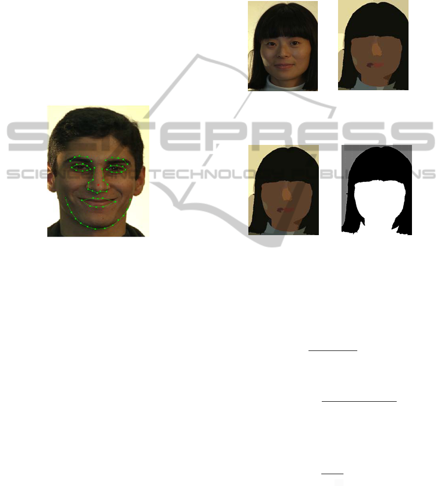
In order to extract the hair features, a hair
segmentation is designed in this study. First, Mean-
shift algorithm roughly classifies a face image
according to the color property, as shown in Figure
2. Then, the segmented image is divided into three
clusters by using k-means clustering, including hair,
face, and background, as shown in Figure 3. Finally,
the hair region is obtained according to the region
area and location. Then, four hair features are
computed: hair length, hair contour length, the ratio
between hair and face lengths, and the complexity of
fringe hair.
(a) (b)
Figure 2: Mean shift segmentation result: (a) original
image, (b) segmented image.
(a) (b)
Figure 3: K-means result: (a) Mean shift segmentation
image, (b) K-means result.
The hair contour can be represented as P={(x
1
,
y
1
), (x
2
, y
2
),…,(x
n
, y
n
)}, (x
i
, y
i
)R
2
, where n denotes
the number of points on the contour. The hair length
is defined as
Hair
len
max
y
i
‐min
y
i
dist
eyes
, (1)
where
eyes
is the distance between eyes. The
hair contour length is defined as
Hair
contour
,
dist
eyes
, (2)
where p
bl
is the lowest point on the left side of the
contour, and p
br
is the lowest point on the right side
of the contour. The ratio between hair and face
lengths is defined as
Hair
ratio
Hair
ed
Hair
len
,
Hair
ed
0
0,
Hair
ed
0
, (3)
where Hair
len
is the hair length feature and Hair
ed
is
the hair length under eyes, as shown in Figure 4. The
complexity of fringe hair is defined as the
GenderClassificationUsingM-EstimatorBasedRadialBasisFunctionNeuralNetwork
303

approximate entropy (ApEn) (Pincus, 1995) of the
lower contour points between P
and P
. ApEn is a
recently developed statistic quantifying regularity
and complexity, and it was widely used in the
physiological time-series analysis. The larger the
ApEn value is, the more complex the fringe is.
Figure 4: Feature of the ratio between hair and face
lengths.
Mustache is the unique feature of male and could
increase the accuracy rate of gender recognition. The
color difference between nose and mustache regions
is used to describe the mustache feature. First, the
RGB mean values on the mustache region and the
RGB mode values on the nose region are calculated.
Then, the difference between these values is
regarded as the feature. The feature vector is
computed as:
Mdif
f
Mean
R
,Mean
G
,Mean
B
,
Mode
R
,Mode
G
,Mode
B
,
(4)
where Mean
R
, Mean
G
, Mean
B
are the RGB mean
values in the mustache region and
Mode
R
, Mode
G
, Mode
B
are the RGB modes in the
nose region, respectively.
2.3 M-Estimator Based Radial Basis
Function Neural Network
RBF networks have been successfully used as a
classifier in many kinds of applications. The
conventional learning rules of RBF networks are
based on the LMS criterion, which minimize the
quadratic function of the residual errors.
The output of the RBF network is described by
N
k
kkkk
wfy
1
,)(
cxx
, (5)
where y is the actual network output, xR
m1
is an
input vector signal, with individual vector
components given as x
j
, for j=1, 2, …,m, that is,
x=[x
1
, x
2
, …, x
m
]
T
R
m1
. w=[ w
1
, w
2
, …, w
N
]
T
R
N1
is the vector of the weights in the output layer, N is
the number of neurons in the hidden layer, and
k
()
is the basis function of the network from R
m1
to R.
c
k
=[ c
k1
, c
k2
, …, c
km
]
T
R
m1
is called the center
vector of the kth node,
k
is the bandwidth of the
basis function
k
(), and |||| denotes the Euclidean
distance. For each neuron in the hidden layer, the
Euclidean distance between its associated center and
the input to the network is computed. The output of
the neuron in a hidden layer is a nonlinear function
of the distance, and the Gaussian function is widely
selected as the nonlinear basis function. After
computing the output for each neuron, the output of
the network is counted as a weighted sum of the
hidden layer outputs.
A common optimization criterion is used to
minimize the LMS between the actual and desired
network outputs. LMS error function is defined as
(6),
(6)
where r
n
= d(n)- y(n) represents the residual error
between the desired, d(n), and the actual network
outputs, y(n). n indicates the index of the data.
The cost function can be defined as an ensemble
average errors,
)()(
n
rEJ
(7)
where
is one of the parameter sets of the network.
According to the gradient descent method, the
gradient of the cost function J(
) needs to be
computed. The gradient surface can be estimated by
taking the gradient of the instantaneous cost surface.
That is, the gradient of J(
) is approximated by Eq
(8)
n
n
n
r
r
r
J
J
)(
)(
)(
(8)
where
n
n
n
r
r
r
)(
(9)
and
yr
n
(10)
The update equation for the network parameters
is given by
y
rnJnn
n
)()()()1(
(11)
However, LMS is not a good criterion for some
training patterns in which there exist huge errors by
the presence of outliers. Those errors cause the
training patterns move far away from the underlying
2
2
1
)(
nn
rr
SIGMAP2014-InternationalConferenceonSignalProcessingandMultimediaApplications
304

position because the influence function in LMS
criterion is linearly with the size of its error.
Among several methods, which deal with the
outlier problem, M-estimator techniques (Huber,
1984) are the most robust and have been applied in
many applications. M-estimators use some cost
functions which increase less rapidly than that of
least square estimators as the residual departs from
zero. When the residual error increases over a
threshold, M-estimators suppress the response
instead. This work employs Welsch M-estimator
function as the error function, given by
(12)
where
is a scale parameter. The cost function of
RBF network
Eq. (7) can be rewritten as
(13)
where
is one of the parameter sets of the network.
According to the gradient descent method, the
update equation for the network parameters (11) also
can be derived according to (13).
According to the M-estimator behaviour, the
modified RBF networks are able to eliminate the
influence of outliers. In this way, the classification
performance can be improved.
3 EXPERIMENTAL RESULTS
This research uses the Facial Recognition
Technology (FERET) (Phillips, 1998) database to
evaluate the performance. We select 600 frontal face
images from the FERET database. There are 300
images for training and other images for testing.
Table 1: Comparison of other methods.
Methods Accuracy (%)
Shan, C. [14] 94.81
Yuchun, Fang [15] 92.16
Qiu, Huining [17] 92.45
Mehmood, Y. [18] 94
Our method (M-estimator RBF) 94.7
Our method (Traditional RBF) 91.02
To investigate the performance of the PCA
dimensionality reduction, different dimensionalities
are performed which are ranged from 10 to 130
dimensions. The best accuracy rate of the proposed
method achieves 94.7% while the dimensionality is
60, and the number of neurons in RBF network is set
to 12. A comparison of other methods is listed in
Table 1. On the other hand, the table also shows that
the result of our method using traditional RBF
network is only 91.02 % accuracy. It demonstrates
the tolerance to outliers of M-estimator.
4 CONCLUSIONS
This research proposes three types of effective
features, including facial texture features, hair
geometry features, and mustache features, to
perform the gender classification. These features
cover the global, local, geometry, and texture
properties. We also design an M-estimator based
RBF neural network to classify the gender. The
experimental results show that the proposed method
produces a good performance.
ACKNOWLEDGEMENTS
We thank the National Science Council (Grant
number: NSC 102-2221-E-155 -070) for funding
this work.
REFERENCES
Alexandre, L. A., 2010. Gender recognition: A multiscale
decision fusion approach. Pattern Recognition Letters,
31, 1422-1427.
Moghaddam, B. and Ming-Hsuan, Y., 2000. Gender
classification with support vector machines. In
Proceedings of the Fourth IEEE International
Conference on Automatic Face and Gesture
Recognition, 306-311.
Len, B. et al, 2011. Classification of gender and face based
on gradient faces. In Proceedings of the 2011 3rd
European Workshop on Visual Information Processing
(EUVIP), 269-272.
Ueki, K. et al., 2004. A method of gender classification by
integrating facial, hairstyle, and clothing images. In
Proceedings of the 17th International Conference on
Pattern Recognition, 446-449.
Viola, P. and Jones, M., 2001. Rapid object detection
using a boosted cascade of simple features. In
Proceedings of the 2001 IEEE Computer Society
Conference on Computer Vision and Pattern
Recognition, I-511-I-518.
Stegmann, M. B. et al., 2003. FAME-a flexible appearance
modeling environment. IEEE Transactions on Medical
Imaging, 22, 1319-1331.
Chng, E. S. et al., 1996. Gradient radial basis function
networks for nonlinear and nonstationary time series
prediction. IEEE Trans. Neural Networks, 7(1), 190-
194.
2
2
/exp1
2
)(
nnW
rr
)()(
nW
rEJ
GenderClassificationUsingM-EstimatorBasedRadialBasisFunctionNeuralNetwork
305

Leung, H. et al., 2001. Prediction of noisy chaotic time
series using an optimal radial basis functions neural
network. IEEE Trans. Neural Networks, 12(5), 1163-
1172.
Li, C. et al., 2004. Nonlinear time series modeling and
prediction using RBF network with improved
clustering algorithm. in Proc. IEEE Int. Conf. Syst.,
Man, Cybern., 4, 3513-3518.
Wang, Y. et al., 2005. Time series study of GGAP-RBF
network: predictions of Nasdaq stock and nitrate
contamination of drinking water. in Proc. IEEE Int.
Joint Conf. Neural Networks, Montreal Canada, July
3127-3132.
Huber, P. J., 1984. Robust Statistics. John Wiley and Sons,
New York.
Pincus, S. 1995. Approximate entropy (ApEn) as a
complexity measure. Chaos: An Interdisciplinary
Journal of Nonlinear Science, 5, 110-117.
Phillips, P. J. et al, 1998. The FERET database and
evaluation procedure for face-recognition algorithms.
Image and Vision Computing, 16, 295-306.
SIGMAP2014-InternationalConferenceonSignalProcessingandMultimediaApplications
306
