
An Ordering Procedure for Admissible Network Configurations to
Regularize DFR Optimization Problems in Smart Grids
A. Rizzi, F. Possemato, S. Caschera, M. Paschero and F. M. Frattale Mascioli
Dipartimento di Ingegneria dell’Informazione, Elettronica e Telecomunicazioni (DIET)
SAPIENZA University of Rome, Via Eudossiana 18, 00184, Rome, Italy
Keywords:
Distribution Feeder Reconfiguration, Power Factor Correction, Power Losses Minimization, Smart Grid,
Graph Theory, Optimization, Genetic Algorithm.
Abstract:
The power loss reduction is one of the main targets for any electrical energy distribution company. In this paper
the problem of the joint optimization of both topology and network parameters in a real Smart Grid is faced.
A portion of the Italian electric distribution network managed by the ACEA Distribuzione S.p.A. located in
Rome is considered. It includes about 1200 user loads, 70 km of Medium Voltage (MV) lines, 6 feeders,
a Thyristor Voltage Regulator (TVR) and 6 distributed energy sources (5 generator sets and 1 photovoltaic
plant). The power factor correction (PFC) is performed tuning the 5 generator sets and setting the state of the
breakers in order to perform the distributed feeder reconfiguration (DFR). The joint PFC and DFR problem
is faced by considering a suited objective function and by adopting a genetic algorithm. In this paper we
present a heuristic method to compare the graphs of two admissible topologies, such that similar graphs are
characterized by close active power loss values. This criterion is used to define a suited ordering of the list
of admissible configurations, aiming to improve the continuity of the fitness function to the variation of the
configurations parameter. Testsareperformed by feeding the simulation environment with real data concerning
dissipated and generated active and reactive power values. Preliminary results are very interesting, showing
that, for the considered real network, the proposed ordering criteria for admissible network configurations can
facilitate the optimization process.
1 INTRODUCTION
The wide diffusion of Distributed Generation (DG)
represents a possible development of modern electri-
cal distribution systems that can evolve towards Smart
Grids (SG). It can be stated that a SG is a new gen-
eration electrical network where smartness, dynam-
icity, safety and reliability are achieved through the
use of Information and Communication Technologies
(ICT) (Dahu, 2011). Recently, electrical distribution
networks have grown quickly and the backbones of
the existing infrastructures have been built when DG
was not considered at all. As a consequence, elec-
tric power is distributed to the final user through a
unidirectional transportation infrastructure. This con-
figuration implies a considerable transportation con-
sumption due to the long distance between producers
and consumers. The main problems concerning actual
networks are listed below:
• losses due to long distance between producers and
users
• management of energetic flows
• inefficient use of DG related to renewable energy
generators
• lag in the reaction time in case of blackout
• incomplete and inaccurate knowledge on the in-
stantaneous status of the infrastructure
In order to overcome these drawbacks, a large number
of sensors must be installed on the network to obtain
a complete information on the instantaneous status of
the infrastructure. This information can be used as
input of an optimization control algorithm capable of
determining in real time the best network configura-
tion able to satisfy the instantaneous power request
and to drive suitable actuators, optimizing a given ob-
jective function.
The number of DG units in electrical distribution
networks has been increasing very fast in the last few
years (Singh et al., 2011). Technologies used for DG
applications could include non-renewable energy re-
sources, such as internal combustion engines, com-
273
Rizzi A., Possemato F., Caschera S., Paschero M. and Frattale Mascioli F..
An Ordering Procedure for Admissible Network Configurations to Regularize DFR Optimization Problems in Smart Grids.
DOI: 10.5220/0005127302730280
In Proceedings of the International Conference on Evolutionary Computation Theory and Applications (ECTA-2014), pages 273-280
ISBN: 978-989-758-052-9
Copyright
c
2014 SCITEPRESS (Science and Technology Publications, Lda.)

bined cycles, combustion turbines as well as micro-
turbines and renewable energy resources, for example
photovoltaic and wind turbines.
Another important degree of freedom that can be
used to minimize active power loss in distribution
feeders is offered by the opportunity to perform the
distribution feeders reconfiguration (DFR). This oper-
ation consists in switching a certain number of break-
ers, altering the topological structure of the network
considering the topological contraints. Therefore, the
DFR problem can be conceptualized as the task of
choosing the status of network breakers resulting in
the configuration with minimal power losses, while
all the system constraints are satisfied. The main
drawback of DFR is that it results in a complex non-
linear combinatorial problem, since the status of the
switches is non-differentiable. This discontinuous be-
haviour makes the optimization problem related to
DFR very hard to solve. In recent years, many re-
searchers have proposed interesting solutions. Prob-
ably the first contribution in this direction can be
found in (Merlin and Back, 1975), where a branch and
bound type optimization technique is used in order to
find the minimal loss operating configuration, for the
distribution system, at a specific load condition. Af-
ter this work, a few different techniques are proposed
by many researchers (Civanlar et al., 1988), (Carreno
et al., 2008). In recent years, new heuristic algorithms
are proposed in the literature with good results. Prob-
ably, the first attempt to use genetic algorithms (GAs)
to solve the DFR problem with minimal losses can be
found in (Nara et al., 1992). Since then, a great num-
ber of publications based on evolutionary algorithms
are proposed in the literature (Storti et al., 2013a),
(Possemato et al., 2013). Recently, GA is also used
to solve the DFR problem with DG (Chandramohan
et al., 2010), (Storti et al., 2013b). One of the main
difficulties for solving the DFR problem using evolu-
tionary algorithms is the radiality constraint. A solu-
tion to this problem is proposed in (Storti et al., 2014)
where a cooperation with ACEA Distribuzione S.p.A.
is engaged with the aim to design a control strategy
for the SG under development in the west area of
Rome. The authors conclude that the DFR is a chal-
lenging problem do to high non linearity of the objec-
tive function. For this reason, in this paper we propose
an heuristic method based on the Hamming distance
between network configurations, to improve the regu-
larity of the objective function. The rest of the paper
is organized as follows: in section 2 we present the
main characteristics of the SG under analysis, in sec-
tion 3 we formulate the DFR optimization problem,
then in section 4 we describe an ordering criteria for
the network configurations. Finally, in section 5 we
report the results obtained by applying the proposed
ordering heuristic to the set of admissible configura-
tions together with a GA. Moreover, we compare re-
sults of the genetic optimization of network topology
and DGs parameters for the ACEA SG, in the cases
of unordered (Storti et al., 2014) and ordered config-
urations.
2 NETWORK SPECIFICATIONS
The portion of the network we consider in this paper
is located in the west area of Rome. The entire SG is
made up of:
• 5 feeders at 20 kV
• 1 feeder at 8.4 kV
• 2 High Voltage (HV) substations
• 76 Medium Voltage (MV) substations
• 5 generator sets (DGs)
• 1 photovoltaic generator (DG)
• 1 thyristor voltage regulator (TVR)
• 106 three-phase breakers
• 70 km of cables
• 1200 user loads
In each HV substation there is a transformer with 150
kV at the primary winding and 20 kV at the secondary
winding (HV/MV transformer). The cables, the pho-
tovoltaic plant, the MV substations and the TVR are
located in the MV portion of the network, whereas the
user loads and the 5 generator sets are located in the
LV portion of the network.
The TVR is a series voltage compensation device.
It performs a bi-directional voltage regulation that
maintains the system voltage within specified ranges.
The bi-directional relation between the input and the
output voltage is defined as follows:
V
out
= V
in
+ N
tap
∆V N
tap
∈ {0, ±1,±2,±3} (1)
where the values of V
in
and V
out
are expressed in kV
and the ∆V is 0.1 kV. The voltage rated value of V
in
is 8.4 kV. Each MV substation is equipped with 2
breakers (switches) that allow it to connect with the
network in different ways. By changing the state of
these switches it is possible to modify the topology of
the network.
3 PROBLEM FORMULATION
In this paper, we consider the joint PFC and DFR
problem for minimum active power losses, satisfying
ECTA2014-InternationalConferenceonEvolutionaryComputationTheoryandApplications
274

constraints on nodes voltage and branches current as
well as system operating constraints.
3.1 Optimization Procedure
In this section we formulate the problem of active
power losses minimization in SGs. It consists in
finding the optimal network parameters and topolog-
ical configuration that minimize the value of the total
active power losses in the network, considering the
constraints imposed on voltages and currents due to
safety or quality of service issues. Consider an admis-
sible set E of the network parameters and a suitable
cost function J : E → R that associates a real number
to each element in E. Formally, the problem consists
in minimizing the function J in E. Mathematically we
can express the cost function J as follows:
J(k) =
P
loss
(k)
P
gen
(k)
=
P
gen
(k) − P
load
P
gen
(k)
(2)
where k represents an instance of the network pa-
rameters, P
gen
(k) is the total power generated by all
sources, P
load
is the total power absorbed by the loads,
and their difference P
loss
(k) represents the total losses
in the network. Let’s consider a generic SG character-
ized by n real parameters, m integer parameters and p
nominal parameters. We can express the domain of
the ordinal parameters as:
A
′
=
k
′
∈ R
n
× Z
m
: k
′
min
≤ k
′
≤ k
′
max
(3)
in which k
′
min
and k
′
max
represent the vectors of the
minimum and maximum values of the network ordi-
nal parameters k
′
. Concerning the nominal parame-
ters, k
′′
, the domain is a set A
′′
of all possible admis-
sible elements for such parameters:
A
′′
=
k
′′
∈ X
1
× · ··× X
p
(4)
in which X
i
is a generic nominal set with i = 1,..., p.
The overall domain A is defined as A = A
′
× A
′′
and
the parameters vector k is an element of such domain.
Without loss of generality, we consider as possible
to measure the voltages and the currents at all loca-
tions in the network. In order to be valid, a solution k
must satisfy the constraints on voltages and currents
defined below:
B =
k ∈ R
n
× Z
m
× X
1
× · ··× X
p
:
V
min
i
≤ V
i
(k) ≤ V
max
i
,i = 1,..,M
C =
k ∈ R
n
× Z
m
× X
1
× · ··× X
p
:
|I
i
(k)| ≤ I
max
i
,i = 1,..,R
where V
i
(k) is the voltage magnitude of node i for a
fixed instance of parameters k, M represents the num-
ber of nodes, V
min
i
, V
max
i
are the voltage limits for
node i, while |I
i
(k)| represents the current magnitude
of branch i for a particular instance of parameters k, R
the number of branches and I
max
i
the current limit for
branch i. The definitions given above allow to define
the admissible set E as follows:
E = A ∩ B ∩C (5)
This formulation is an example of mixed-integer
black box-based optimization problem because the
optimization variables are integer and real. Moreover,
it is not practically possible to derive expression (2) in
closed form as a function of k; for this reason we em-
ploy a GA (derivative free approach) as optimization
algorithm. The constrained optimization problem is
faced by defining the objective function as a convex
combination of two competitive terms:
F(k) = αJ(k) + (1− α)Γ(k) (6)
where α is a real number in the range [0, 1] used to ad-
just the relative weight of the power losses term J(k)
over the constraints term Γ(k). The function Γ(k) is
defined as follows:
Γ(k) = (1− β)Γ
I
(k) + βΓ
V
(k) (7)
in which β is a real number in the range [0, 1] used
to adjust the relative weight of the violation of current
constraints Γ
I
(k) with respect to the term related to
voltages violation Γ
V
(k). In this paper it is performed
the minimization of F(k) in A. Further details of the
optimization procedure can be found in (Storti et al.,
2013a).
3.2 Admissible Network Configurations
In order to perform the optimization procedure de-
scribed in section 3.1, we introduce a suitable repre-
sentation of the SG as a non oriented graph GhN,Ei,
in which N and E are the nodes and the edges of the
real network, respectively. Let’s define as
ˆ
Gh
ˆ
N,
ˆ
Ei,
the reduced graph of the network. The objective
of this representation is to properly describe all the
possible system reconfigurations satisfying the topol-
ogy constraints. The reduced graph of the network
ˆ
Gh
ˆ
N,
ˆ
Ei doesn’t contain all the information of the
original network graph GhN,Ei because for our pur-
poses we need only to know how different portions
of the network can be electrically connected. As de-
scribed in (Storti et al., 2014), the mapping of the real
network in the simplified graph version is performed
through two main steps:
• The nodes
ˆ
N of the simplified graph are used to
model 2 different types of original nodes N. The
first one represents nodes at 150kV providing the
energy balance of the active and reactive power
AnOrderingProcedureforAdmissibleNetworkConfigurationstoRegularizeDFROptimizationProblemsinSmartGrids
275

in the SG. In following sections we will refer to
it as HV node. The second one can represent a
single MV real substation eventually connected to
loads, DGs and TVR, or a set of MV substations,
powered by a single HV substation only (virtual
MV). In both cases, we call this kind of nodes as
MV node.
• Edges
ˆ
E of the reduced network graph are used to
model the topology reconfiguration. The series of
two switches, installed between two consecutive
MV substations, are mapped into a single edge of
the reduced graph
ˆ
G (virtual breaker). Each edge
is associated with a label representing its state i.e.
close or open.
Figure 1 shows an example of the representation of
the network through the reduced graph
ˆ
Gh
ˆ
N,
ˆ
Ei.
Using the above notation we can introduce the fol-
lowing definitions:
Def. 1 (Radial Topology Constraint). A network
topology satisfies the Radial Topology Constraint iff
each MV substation is fed by only one HV substation
via only one path.
Def. 2 (Admissible Configuration). A reduced
graph
ˆ
Gh
ˆ
N,
ˆ
Ei satisfying the radial topology con-
straint is said to be an admissible configuration of the
network.
The graph representation
ˆ
Gh
ˆ
N,
ˆ
Ei is used to per-
form an algorithm that executes an exhaustive search
of all the admissible configurations of the network.
The details of the automatic procedure are described
in (Storti et al., 2014). The output of such procedure
is a list of binary strings (admissible configurations)
having length equals to the number of edges
ˆ
E of
the reduced network graph. Each bit represents the
state of the corresponding edge (breaker). The net-
work topology is specified by an integer index, named
N
conf
, spanning the rows of the list of admissible con-
figurations ordered according to the automatic proce-
dure. During the optimization procedure, N
conf
con-
stitutes a nominal parameter to be optimized, so the
objective function can change abruptly moving from
a given configuration to the previous or the next one,
making very challenging this optimization due to high
discontinuities in the objective function. For this rea-
son, in the following section, we present an heuris-
tic method to compare the graphs of two admissi-
ble topologies, in terms of active power loss values
through a purely topological analysis. This criterion
is used to define a suited ordering of the list of admis-
sible configurations, aiming to improve the continuity
of the objective function to the variation of the N
conf
parameter.
HV
MV
MV
MV
MV
MV
MV
MV
MV
MV
MV
MV
MV
MV
MV
HV
MV
MV
Figure 1: Example of the graph
ˆ
Gh
ˆ
N,
ˆ
Ei of the simplified
network. Orange circlesindicate MV nodes, gray rectangles
are HV nodes, dashed arrows represent open status edges.
The dashed box highlights a portion of the network.
4 ORDERING HEURISTIC
In order to make effective any algorithm for solv-
ing the optimization problem described in section 3.1,
we need an ordering heuristic of the admissible con-
figurations to improve the ’regularity’ of the objec-
ECTA2014-InternationalConferenceonEvolutionaryComputationTheoryandApplications
276

tive function. In such a derivative free mixed inte-
ger context, it means reducing the variations of the
objective function evaluated at an admissible config-
uration i from the objective values at i − 1 and i + 1,
for i = 2,3,... ,n − 1, where n indicates the number
of the admissible configurations found as described
in the previous section.
4.1 Graph Representation of
Admissible Network Configurations
Each admissible configuration of the network is iden-
tified by a binary string of length equal to the num-
ber of virtual breakers of the reduced graph. Given
a pair of configurations hi, ji, we use the Hamming
distance between the respective bit strings, d
H
(i, j),
to quantify the dissimilarity between i and j. Let
D be a square matrix of order n containing all the
Hamming distances between admissible configura-
tions, i.e. d
ij
= d
H
(i, j) for i, j = 1, ...,n. Of course D
is symmetric with zeros along the diagonal only. Let’s
define as G
AC
the undirected graph of the admissible
configurations represented by D, where each element
d
ij
of the matrix is the weight w
ij
of the edge e
ij
that
connects nodes i and j of G
AC
. Let’s denote by N
AC
and E
AC
the sets of nodes and edges of G
AC
, respec-
tively. Figure 2 shows an example of the building pro-
cess of G
AC
. The portion of the reduced graph con-
sidered in the example is highlighted within a dashed
box in Figure 1. Opening the virtual breaker between
nodes
ˆ
N
3
and
ˆ
N
4
represented by edge
ˆ
E
3,4
, we ob-
tain the configuration [1 1 0 1], while disconnecting
nodes
ˆ
N
2
and
ˆ
N
3
and reconnecting nodes
ˆ
N
3
and
ˆ
N
4
by opening the virtual breaker
ˆ
E
2,3
and closing
ˆ
E
3,4
,
the resulting configuration is [1 0 1 1]. The extracted
configurations are two nodes of the graph G
AC
at dis-
tance d
H
= 2.
4.2 Heuristic method for ordering the
admissible configurations
In this subsection we present an heuristic method,
based on G
AC
, used to order the admissible configu-
rations of the network to avoid strong discontinuities
between active power loss values of consecutive con-
figurations. Then, in section 5 we will show how this
method applied to a real electrical network actually
makes less difficult to solve the optimization problem
presented in section 3.1.
Given a configuration i, the objective function value
F(k) will depend on all the other parameters values
in k, i.e. on a set of virtually infinite combinations.
However we need to associate with each configura-
tion a unique scoring function, as an average estimate
ˆ
N
1
ˆ
N
2
ˆ
E
1,2
ˆ
N
3
ˆ
E
2,3
ˆ
N
4
ˆ
E
3,4
ˆ
N
5
ˆ
E
4,5
ˆ
N
1
ˆ
N
2
ˆ
E
1,2
ˆ
N
3
ˆ
E
2,3
ˆ
N
4
ˆ
E
3,4
ˆ
N
5
ˆ
E
4,5
ˆ
Gh
ˆ
N,
ˆ
Ei
1101 1011
d
H
= 2
G
AC
hN
AC
,E
AC
i
Figure 2: Building process of configurations graph G
AC
of
a portion of two instances of the reduced network graph
ˆ
Gh
ˆ
N,
ˆ
Ei.
of F(k). To this aim, the following reference values of
the real parameters are chosen for all configurations:
(
k
j
) = (k
j,min
+ k
j,max
)/2, j = 1,.. ., n (8)
and for the integer parameters:
(
k
h
) = [(k
h,min
+ k
h,max
)/2], h = 1,.. .,m (9)
in which the operator [·] indicates the round opera-
tion. For simplicity we will refer to f(i) to indicate
F(k)|
N
conf
=i
and to
¯
f(i) to represent the fitness f(i)
computed in the reference values of the parameters
expressed in (8) and (9).
Let W be the list of all possible values for the weights
of the edges of graph G
AC
, ordered in ascending man-
ner:
W = [w
1
,w
2
,. .., w
m
]
Fixed a node i of G
AC
and a weight w
j
∈ W, we de-
fine (N
AC
i
)
w
j
as the set of all nodes connected with i
by edges with weight w
j
. An estimate of the differ-
ence between
¯
f(i) at i-th node and the objective val-
ues associated with the nodes belonging to (N
AC
i
)
w
j
,
is given by the mean distance (∆F
i
)
w
j
between
¯
f(i)
and the fitness
¯
f(k), ∀k ∈ (N
AC
i
)
w
j
. Indicating as
(∆
¯
f
i,k
)
w
j
=
¯
f(i)−
¯
f(k)
/
¯
f(i) the relative distance be-
tween the fitness
¯
f(i) and the fitness
¯
f(k), the mean
distance can be mathematically expressed as:
(∆F
i
)
w
j
=
∑
(l
i
)
w
j
k=1
(∆
¯
f
i,k
)
w
j
(l
i
)
w
j
(10)
where (l
i
)
w
j
is the cardinality of (N
AC
i
)
w
j
. If each
node i of G
AC
satisfies the following property:
(∆F
i
)
w
1
≤ (∆F
i
)
w
j
, j = 2,.. .,m (11)
AnOrderingProcedureforAdmissibleNetworkConfigurationstoRegularizeDFROptimizationProblemsinSmartGrids
277

we can deduce that, in mean, the active power loss
of the network varies less between similar configura-
tions than between dissimilar ones. Remember that
with ’similar’ we indicate similarity in terms of Ham-
ming distance. We can extract the subgraph G
AC
w
1
=
hN
AC
,E
AC
w
1
i, whose set of edges E
AC
w
1
is defined as fol-
lows:
E
AC
w
1
= {e
ij
∈ E
AC
s.t. w
ij
= w
1
, (12)
∀i, j = 1, 2,...,n}
The existence of an edge between a pair of nodes i
and j of the graph G
AC
w
1
should indicate that the con-
figurations i and j have close active power losses. In
the following section we will proof such property for
the network under analysis.
To order the admissible configurations of the network
we use the depth first traversal algorithm on G
AC
w
1
. The
order in which the nodes are visited will be the new
sequence of the indexes of the admissible configura-
tions.
5 TESTS AND RESULTS
In this section we first empirically prove the property
expressed in (11) for the network under consideration,
then we compare the performances of GA when it
is used to solve the optimization problem presented
in section 3.1 for the considered electrical network,
whether the configurations are ordered or unordered.
Following the notation introduced in section 3.1
and network specifications described in section 2, we
can control the reactive power of the 5 generator sets
through the phase parameters φ. Instead it is not pos-
sible to control the reactive power of the photovoltaic
generator. Moreover it is possible to chose the N
tap
value of the TVR and the configuration of the net-
work selecting it from the set of admissible ones pre-
viously determined. The phases of the 5 generator
sets φ
1
,φ
2
,φ
3
,φ
4
,φ
5
will be spanned in a real given
range specified by the capability functions of the cor-
responding generator sets. The tap N
tap
of the TVR
will be spanned in the discrete (normed) range de-
fined in (1). Finally,according to the list of admissible
configurations introduced in section 3.2, the network
topology is specified by an index, N
conf
, spanning the
rows of such list. In particular, in the smart grid un-
der consideration, the number of admissible configu-
rations is 390. Summarizing, the candidate solution
vector k = [φ
1
,φ
2
,φ
3
,φ
4
,φ
5
,N
tap
,N
conf
] will span the
set defined below:
A = { k ⊂ R
5
× Z × X : −0.2 ≤ φ
1
,φ
2
≤ 0.45
−0.2 ≤ φ
3
≤ 0.55
0.0 ≤ φ
4
≤ 0.64
−0.32 ≤ φ
5
≤ 0.45
−3 ≤ N
tap
≤ 3
N
conf
∈ X }
in which X = {conf
1
,..., conf
390
} is the set of indexes
of all configurations. Moreover, in order to be valid,
a solution k must satisfy the constraints on voltages
and currents defined below:
B =
k ⊂ R
5
× Z × X : 0.9V
nom
j
≤ V
j
(k) ≤ 1.1V
nom
j
, j = 1, ..,M
C =
k ⊂ R
5
× Z × X : |I
j
(k)| ≤ I
max
j
, j = 1,..,R
in which M and R represent the total number of
nodes and branches of the real network, respectively,
whereas V
nom
j
and I
max
j
are the nominal value of the
voltage of the j-th node and the maximum current al-
lowed in the j-th wire, respectively.
Performing the analysis described in the previous
section, we found that in the network under consid-
eration there are only three different possible weights
(i.e. Hamming distance values) associated with the
edges of the graph of the admissible configurations
G
AC
. In particular:
W = [2,4,6]
whereby we have to compute (∆F
i
)
2
, (∆F
i
)
4
, (∆F
i
)
6
for i = 1,2,. .. ,390. The minimum weight belong-
ing to W is w
min
= 2, as we could expect, since in
a real electrical network, a topology change implies,
at least, closing a given breaker and opening another
one. Thus, we have to check if the following two con-
ditions are satisfied:
(∆F
i
)
2
≤ (∆F
i
)
4
i = 1,...,390 (13)
(∆F
i
)
2
≤ (∆F
i
)
6
i = 1,...,390 (14)
To compute the fitness value associated with each
node of G
AC
, we have considered as input of the
network model the power profile associated with the
1:00PM (one hour) of the 1-st of January.
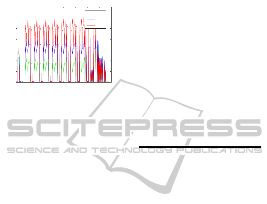
Figure 3 shows the values of (∆F
i
)
2
, (∆F
i
)
4
, (∆F
i
)
6
calculated for all nodes of G
AC
. It is possible to ob-
serve that, for most of nodes, relations (13) and (14)
are satisfied. An accurate data analysis returns that
over 97% of nodes (network configurations) satisfy
these two relations.
It’s important to point out that this result doesn’t de-
pend on the values initially assigned to fitness param-
eters
φ
j
for j = 1,.. .,5 and N
tap
. In fact, the set of
nodes satisfying relations (13) and (14) is the same for
any set of admissible values initially assigned to these
ECTA2014-InternationalConferenceonEvolutionaryComputationTheoryandApplications
278
0 50 100 150 200 250 300 350 400
0
20
40
60
80
100
120
140
nodes i=1,2,...,390
(∆F
2
)
i
(∆F
4
)
i
(∆F
6
)
i
Figure 3: Mean distance between the fitness value associ-
ated with node i,
¯
f(i), and fitness values associated with
all the adjacent nodes of the i-th node belonging to (N
AC
i
)
2
,
(N
AC
i
)
4
, (N
AC
i
)
6
respectively, for i = 1,2, ... ,390. The scale
factor is equal to
¯
f(i).
parameters. Thus, we have empirically proven Equa-
tion (11), specifically that similar network configura-
tions (i.e. nodes of graph G
AC
connected by edges
with small weights) correspond to close active power
loss values. Note that we have verified this property
only for the network under analysis.
At this point, as described in section 4.2, we
can choose a depth first traversal of the sub graph
G
AC
2
hN
AC
,E
AC
2
i to order the admissible configura-
tions. It was verified that G
AC
2
is a connected graph,
with size, i.e. the number of its edges, equal to 4743.
In particular, the minimum degree of G
AC
2
, i.e. the
minimum number of edges incident to its nodes, is
equal to 21. There are 90 nodes having this num-
ber of edges incident to them. The maximum degree
of G
AC
2
is 37 and only 20 nodes have this number of
edges incident to them. In order to compare the effec-
tiveness of this ordering heuristic technique in solving
the proposed optimization problem, the execution of
GA is repeated 6 times, whether the configurations
are ordered or unordered. Different executions con-
sider different sequences of indexes obtained through
depth first traversal of G
AC
2
, starting from different
root nodes.
To compare performances of GA, the algorithm
parameter setting is chosen identical whether the con-
figurations are ordered or unoredered (in the second
case, we consider the initial ordering of the admis-
sible configurations returned by the automatic proce-
dure described in (Storti et al., 2014)). In particular,
the number of individuals of a population is set to 20.
The elite individuals are 2, i.e. only 2 individuals in
the current generation are guaranteed to survive to the
next generation. The crossover fraction parameter is
0.8. The mutation operator is applied to the remain-
ing individuals. Furthermore, the α and β coefficients
used in expressions (6) and (7) are set to 0.9 and 0.2,
respectively.
The maximum number of iterations before the algo-
rithm halts is 100, but GA can stop if the weighted
average relative change in the fitness value over 50 it-
erations is less than or equal to 10
−9
.
All performed tests consider the same states of the
network to seed GA. More precisely, a fixed initial
population is considered for all of the executions of
the GA when the admissible configurations are or-
dered and unordered. It should be noted that the ran-
dom initialization does not necessarily ensure the sat-
isfaction of the constraints consideredin the definition
of the chosen fitness function. Results of the simu-
Table 1: Mean number of generations (# gen) produced by
GA to return the optimal solution, mean percentage reduc-
tion of the fitness value (%F reduct.), mean reduction of the
active power loss (P
loss
) whether the admissible configura-
tions are ordered or unordered.
ordered conf. unordered conf.
# gen 73 67
%F reduct. 0.023 0.022
P
loss
reduct. [W] 1096.97 1088.34
lations are shown in Table 1. It compares the mean
value of the number of generations created (#gen),
the fitness percentage reduction (%F reduct.) and the
reduction of active power loss of the network (Ploss
reduct.), whether the configurations are ordered or un-
ordered (Storti et al., 2014). More precisely, last two
indicators consider the reduction of the fitness value
and actual active power loss between the optimal so-
lution and the best individual of the initial population.
Moreover, Figures 4 (a)-(b)-(c) show the mean value
of the number of generations, the mean percentage
reduction of fitness value and the mean reduction of
power loss and the respective standard deviation in
both cases of ordered and unordered list of configura-
tions.
We can note that the mean number of generations
of GA when the configurations are ordered is larger
than in the unordered case. This is due to greater
headway made by GA during the search process of
the optimal solution, in the first case. This allows to
have, on average, an higher reduction of the fitness
value, as well as of the total active power loss, from
the initial state of the considered network. As we ex-
pected, the power loss reduction is not very high, but
considering that all the tests simulate only one hour
of one day and projecting this power loss reduction
to the whole network over time, the savings could be-
come interesting in the regular operating condition of
the real network in which the value of the power loss
AnOrderingProcedureforAdmissibleNetworkConfigurationstoRegularizeDFROptimizationProblemsinSmartGrids
279

Not Ord. Config. Ord. Config.
0
20
40
60
80
100
Generation
(a)
Not Ord. Config. Ord. Config.
0
0.01
0.02
0.03
Fitness reduction (%)
(b)
Not Ord. Config. Ord. Config.
0
500
1000
1500
AP Loss Reduction [W]
(c)
Figure 4: Mean value of the number of generations (a), the
mean percentage reduction fitness value (b) and the mean
reduction of active power loss (c) with the respective stan-
dard deviation for ordered and unordered list of configura-
tions.
becomes considerable.
6 CONCLUSIONS
In this paper an improvement of the control system
described in (Storti et al., 2013a), (Possemato et al.,
2013), (Storti et al., 2013b) and (Storti et al., 2014) is
presented. We propose an heuristic method to com-
pare admissible network topologies and a criteria to
order the list of such topologies aiming to improve the
continuity of the objective function to the variation of
the configuration parameter. We execute some tests
on the SG sited in the west area of Rome realized by
ACEA Distribuzione S.p.A.. Results show that, for the
network under analysis, the proposed ordering pro-
cedure makes the joint PFC and DFR optimization
problem simpler to cope with a plain genetic algo-
rithm. In future works we intend to verify the criteria
in a more complex network and at different time inter-
vals. Moreover, by exploiting the property described
by Equations 13 and 14, it is possible to redefine more
suitable mutation and crossover operators to furtherly
improve the convergence of the GA during the evolu-
tionary process.
REFERENCES
Carreno, E., Romero, R., and Padilha-Feltrin, A. (2008). An
efficient codification to solve distribution network re-
configuration for loss reduction problem. IEEE Trans-
action on Power Systems, 23(4):15421551.
Chandramohan, S., Atturulu, N., Kumudini, R., and Ven-
takesh, B. (2010). Operating cost minimization of
a radial distribution system in a deregulated electric-
ity market through reconfiguration using nsga method.
International Journal of Electric Power Energy Sys-
tems, 32(2):126132.
Civanlar, S., Grainger, J., Yin, H., and Lee, S. (1988).
Distribution feeder reconfiguration for loss reduc-
tion. IEEE Transactions on Power Delivery,
3(3):12171223.
Dahu, L. (2011). Electric power communication system of
the future smart grid. Telecommunication for Electric
Power System, 32(222).
Merlin, A. and Back, H. (1975). Search for minimum-
loss operational spanning tree configuration for urban
power distribution systems. In Proceeding of Fifth
power system conference (PSCC), page 118.
Nara, K., Shiose, A., Kitagawa, M., and Ishibara, T. (1992).
Implementation of genetic algorithm for distribution
systems loss minimum reconfiguration. IEEE Trans-
action on Power Systems, 7(3):10441051.
Possemato, F., Storti, G., Paschero, M., Rizzi, A., and Frat-
tale Mascioli, F. (2013). Two evolutionary computa-
tion approaches for active power losses minimization
in smart grids. In Proceedings of North America Fuzzy
Information Processing Society.
Singh, M., Khadkikar, V., Chandra, A., and Varma, R.
(2011). Grid interconnection of renewable energy
sources at the distribution level with power-quality
improvement features. IEEE Transactions on Power
Delivery, 26(1):307–315.
Storti, G., Possemato, F., Paschero, M., Alessandroni, S.,
Rizzi, A., and Mascioli, F. F. (2013a). Neural Nets
and Surroundings 22nd Italian Workshop on Neu-
ral Nets, WIRN 2012, May 17-19, Vietri sul Mare,
Salerno, Italy, volume 19 of Smart Innovation, Sys-
tems and Technologies, chapter Active power losses
constrained optimization in Smart Grids by gentic al-
gorithms, pages 279–288. Springer Berlin Heidelberg.
Storti, G., Possemato, F., Paschero, M., and nad F.M. Frat-
tale Mascioli, A. R. (2014). A radial configurations
search algorithm for joint pfc and dfr optimization in
smart grids. In Proceeding of 23th international con-
ference on industrial electrincs (ISIE).
Storti, G., Possemato, F., Paschero, M., Rizzi, A., and Frat-
tale Mascioli, F. M. (2013b). Optimal distribution
feeders configuration for active power losses mini-
mization by genetic algorithms. In Proceedings of
North America Fuzzy Information Processing Society.
ECTA2014-InternationalConferenceonEvolutionaryComputationTheoryandApplications
280
