Trawl-door Shape Optimization with 3D CFD

Models and Local Surrogates

Elvar Hermannsson

, Leifur Leifsson

, Slawomir Koziel

, Piotr Kurgan

and Adrian Bekasiewicz

KTH Royal Institute of Technology, School of Engineering Sciences, Stockholm, Sweden

Engineering Optimization & Modeling Center, Reykjavik University, Menntavegur 1, Reykjavik, Iceland

Faculty of Electronics, Telecommunications and Informatics, Gdansk University of Technology, 80-233 Gdansk, Poland

Keywords: Trawl-Door, Ship Fuel Efficiency, Hydrodynamics, Shape Optimization, 3D CFD.

Abstract: Design and optimization of trawl-doors are key factors in minimizing the fuel consumption of fishing

vessels. This paper discusses optimization of the trawl-door shapes using high-fidelity 3D computational

fluid dynamic (CFD) models. The accurate 3D CFD models are computationally expensive and, therefore,

the direct use of traditional optimization algorithms, which often require a large number of evaluations, may

be prohibitive. The design approach presented here is a variation of sequential approximate optimization

exploiting low-order local response surface models of the expensive 3D CFD simulations. The algorithm is

applied to the design of modern and airfoil-shaped trawl-doors.

1 INTRODUCTION

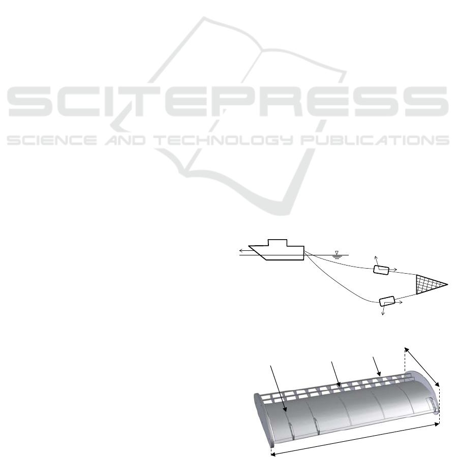
Trawling gear contributes to a majority of the

fuel expenditure of many fishing vessels. Fishing

gear main parts are the net, a pair of trawl-doors, and

a cable extending from the trawl-doors to the boat

and the net (see Fig. 1(a)). The role of the trawl-

doors is to keep the net open during the trawling

operation. Typically, their span is 6-8 m and chord

2-3 m, while the cables are over a few hundred

meters long and the net tens of meters. Figure 1(b)

shows a modern trawl-door. The trawl-doors may be

responsible for roughly 10-30% of the total drag of

the entire assembly (Garner, 1967). Good trawl-door

designs are therefore desired to minimize fuel

consumption.

In general, trawl-doors have remained the same

for many decades. This is mainly due to the fact that

their designs are based on time-consuming and

expensive physical experiments in tow- or flume

tanks. Computational fluid dynamics (CFD) is

widely used for the design of a variety of vehicles.

However, very few CFD-based studies are reported

for trawl-doors in the literature (Haraldsson, 1996).

Recently, a design optimization approach for

trawl-doors using 2D CFD models has been

introduced (Leifsson et al., 2014). The approach can

be categorized as surrogate-based. As a surrogate

model (i.e., a cheaper representation of expensive

CFD simulations) it exploits low-order local

response surface approximations of the sparsely

sampled 2D CFD simulation data.

(a)

(b)

Figure 1: Schematic of a fishing vessel with trawling gear

illustrating (a) the main parts of the fishing gear (not

drawn to scale), and (b) a typical trawl-door with two

slats.

Trawl-doors

Cables

Net

Main Element (ME)

cʹ

Slat 1

Slat 2

775

Hermannsson E., Leifsson L., Koziel S., Kurgan P. and Bekasiewicz A..

Trawl-door Shape Optimization with 3D CFD Models and Local Surrogates.

DOI: 10.5220/0005131307750784

In Proceedings of the 4th International Conference on Simulation and Modeling Methodologies, Technologies and Applications (SDDOM-2014), pages

775-784

ISBN: 978-989-758-038-3

 2014 SCITEPRESS (Science and Technology Publications, Lda.)

2D CFD models are a simplified representation

of the flow past trawl-doors. To perform a more

realistic and practical design of trawl-doors, 3D

CFD models are required to capture the flow physics

more accurately. In particular, the trawl-doors are

low aspect ratio, and, therefore, the tip vortex will

have significant effect on the overall performance.

In this paper, we extend our methodology to use 3D

CFD models, using the optimized 2D design as a

starting point. Although computationally more

expensive, the use of 3D CFD simulations turns out

to be critical for design reliability.

2 PROBLEM FORMULATION

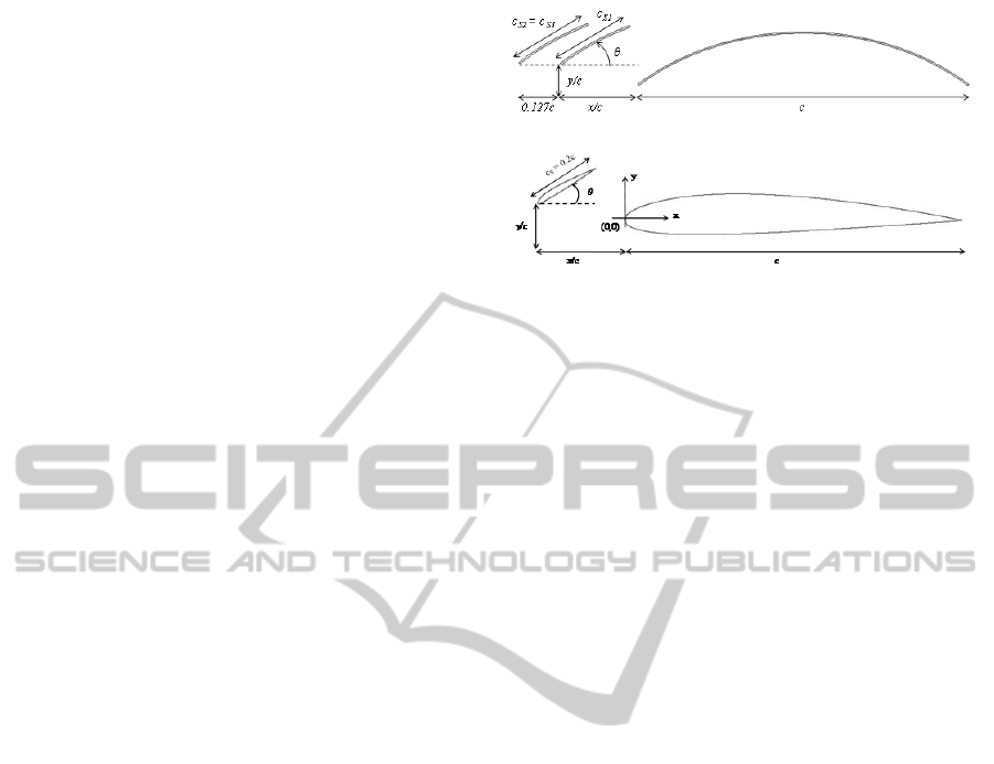
The design goal is to optimize the shape and

configuration of trawl-doors. The design of other

components of the trawling gear is not considered here.

We setup the trawl-doors using a typical modern shape

(Fig. 2(a)) and with airfoil profiles (Fig. 2(b)) as

proposed in our earlier work (Jonsson et al., 2012;

Jonsson et al., 2013).

The objective is to minimize the drag of the 3D

trawl-door while maintaining a given lift to ensure

sufficient opening of the net. In particular, the

optimization problem is formulated as

min 



(1)

subject to









∗

(2)

where C

the drag coefficient (a nondimensional form

of the trawl-door drag), C

is the lift coefficient, and

is the minimum allowable lift coefficient.

The position and inclination of the elements are the

design parameters. The design variable vector can be

written as





/ / 







(3)

where x/c is the slat leading-edge position on the x-axis,

y/c is the slat leading-edge position on the y-axis,



the slat inclination relative to the x-axis,



is the flow

angle of attack relative to the x-axis, and c is the length

of the main element (c = 1 in this study). Upper and

lower bounds, u and l, respectively, are prescribed on

the design variables.

The size and shape of the elements is fixed. The

operating condition, the flow speed V



, is also fixed

during the optimization.

(a)

(b)

Figure 2: Section cuts of the two shapes, (a) a typical

modern trawl-door with thin elements (the F11), and (b) a

novel trawl-door with airfoil shaped elements.

3 CFD MODELS

This section describes the CFD models used in this

study. In particular, we describe the 2D and the 3D

CFD model setup and configuration, as well as give

the results of mesh convergence studies and model

validation.

3.1 Governing Equations

The flow is assumed steady, incompressible, and

viscous. The Reynolds-averaged Navier-Stoke

(RANS) equations are taken to be the governing

equations with Menter’s k-



SST turbulence model

(see, e.g., Tannehill et al., 1997).

3.2 Computational Grid

The farfield is configured in a box-topology where

the trawl-door geometry is placed in the center of the

box. The main element leading edge (LE) is placed

as the origin, with the farfield extending 100 chord

lengths away from the origin in every direction.

Figure 3 shows the 2D solution domain and Fig. 4

shows the 3D one.

The grid is an unstructured triangular one where

the elements are clustered around the trawl-door

geometry, growing in size as they move away from

the origin. The maximum element size on the

geometry is set to 0.1% of the chord length. The

maximum element size in domain away from the

trawl-door is 10 times the chord length. In order to

capture the viscous boundary layer well, a prismatic

inflation layer is extruded from all surfaces. The

initial layer height is chosen so that y

< 1. The mesh

is generated with ICEM CFD (ICEM CFD, 2012).

Example meshes is shown in Figs. 5 and 6.

SIMULTECH2014-4thInternationalConferenceonSimulationandModelingMethodologies,Technologiesand

Applications

776

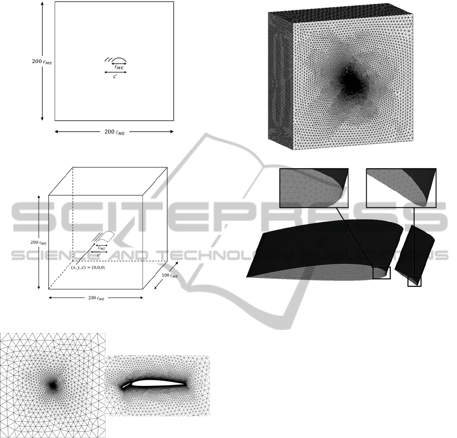
Figure 3: 2D CFD model solution domain.

Figure 4: 3D CFD model solution domain.

(a) (b)

Figure 5: An example 2D computational grid, (a) the

farfield, and (b) a close-up of the trawl-door surface.

3.3 Flow Solver

Numerical fluid flow simulations are performed

using the commercial computer code FLUENT

(FLUENT, 2012). The flow solver is coupled

velocity-pressure-based formulation. A velocity inlet

boundary condition is prescribed to all the edges of

the farfield, aside from the outlet edge which has a

pressure outlet boundary condition.

(a)

(b)

Figure 6: An example 3D computational grid, (a) the

farfield, and (b) a close-up of the trawl-door surface.

The spatial discretization schemes are second

order for all flow variables and the gradient

information is found using the Green-Gauss node

based method. Additionally, due to the difficult flow

condition at high angle of attacks, the pseudo-

transient option and high-order relaxation terms are

used in order to get a stable converged solution. The

residuals, which are the sum of the L

norms of all

governing equations in each cell, are monitored and

checked for convergence. The convergence criterion

is such that a solution is considered to be converged

if the residuals have dropped by six orders of

magnitude, or the total number of iterations has

reached 6,000 for the 2D model and 2,000 for the

3D model.

3.4 Grid Convergence

A convergence study is performed in order to obtain

a grid that is sufficiently fine to capture the flow

physics accurately. The methodology of the study is

to run the CFD model at the same flow conditions,

but with computational grids of various densities.

The CFD model should capture the flow

characteristics with more accuracy when the grid is

Trawl-doorShapeOptimizationwith3DCFDModelsandLocalSurrogates

777

finer. The purpose of the grid convergence study is

then to determine the grid density that results in

stable simulation results (i.e., not changing upon

further grid refinement). The grid satisfying this

condition is considered to be converged with respect

to the discretization density.

The study is conducted for both 2D and 3D CFD

models using a two-element trawl-door

configuration with the main element shape of NACA

2410 and a leading-edge slat shape of NACA 3210

(shown in Figs. 5 and 6). The leading-edge of the

slat is at (x/c,y/c) = (-0.20,-0.08). The slat is inclined



= 35°. The free-stream velocity is set at V

∞

= 2

m/s, the angle of attack at α = 20° and the Reynolds

number is Re = 210

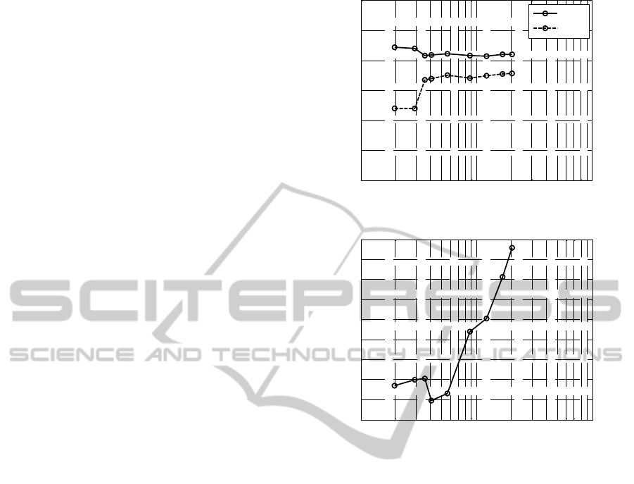
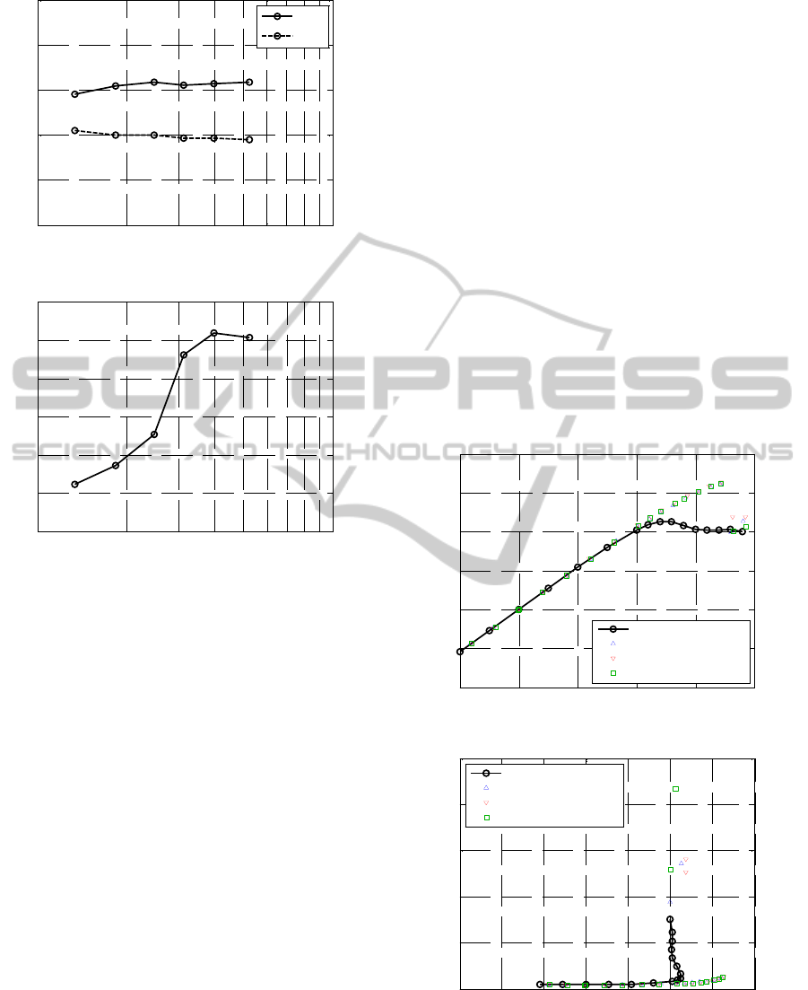
The results of the 2D convergence study shown

in Fig. 7(a) indicate that the grid is converged at

168,592 elements, which is the eighth data point,

counting from the left - the lower boundary of the x-

axis. This grid will be used for the 2D CFD model.

The simulations were executed using four parallel

program nodes, on two Intel Xeon(R) X5660 2.8

GHz processors connected in parallel. The resulting

simulation time needed for each of the data points

are presented in Fig. 7(b). Inspection of Fig. 7(b)

reveals that the simulation runtime decreases

significantly from the third to the fourth data point,

although the element number is higher. As

mentioned before, the convergence criterion is

configured in such way that either all of the residuals

need to be reduced by six orders of magnitude or

that the number of iterations reach up to 6,000. The

solution was converged where all residuals had been

reduced by six orders after less than 2,500 iterations

at the fourth and fifth data points, and that explains

the decreased runtime.

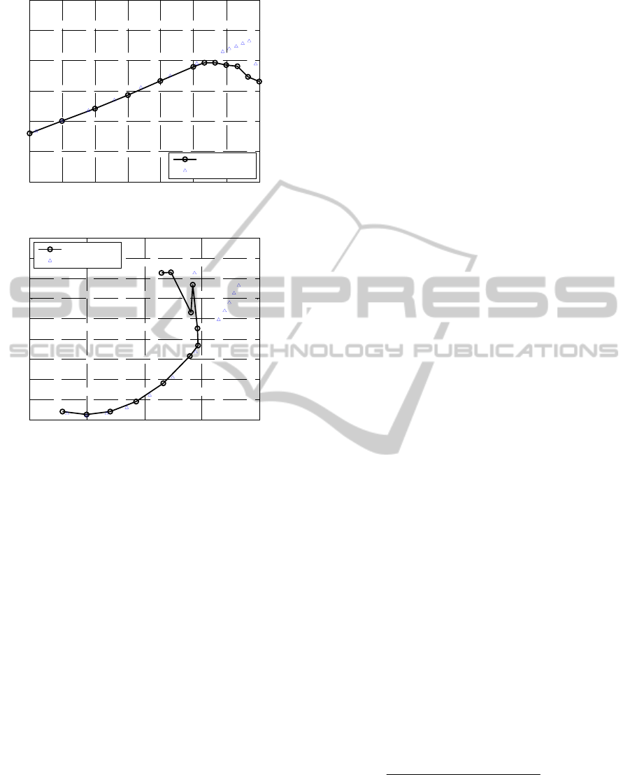
The results of the 3D convergence study shown

in Fig. 8(a) indicate that the grid is converged at

3,972,136 elements, which is the fifth data point,

counting from the left - the lower boundary of the x-

axis. The number of iterations for each of the

simulation runs was 2,000, executed on two Intel

Xeon(R) X5660 processors connected in parallel.

The resulting time needed for each simulation using

the various grids is presented in Fig. 8(b). The

simulation time for the chosen 4 million element

computational grid is therefore around 26 hours. The

simulation time for the sixth data point resulted to be

less than for the fifth one, although the number of

elements is significantly greater. This is caused by

the fact that the solution converged with all residuals

reduced by six orders, before the maximum number

of iterations was reached.

(a)

(b)

Figure 7: Results of a grid convergence study of the 2D

CFD model at V

∞

= 2 m/s and α = 20°; coefficients of (a)

lift and (b) drag versus the number of grid elements.

3.5 Validation

Experimental data is not available for the trawl-door

geometries that are used in this study. Consequently,

other geometries have to be used to validate the CFD

models. For the 2D CFD model, the NACA 0012

airfoil is chosen for the validation process using the

data from Ladson (1988). The 3D CFD model is

compared against the data by Whicker and Fehlner

(1958).

Results for the lift and drag coefficients from the

2D CFD model, compared with the tripped data

from Ladson (1988) are presented in Fig. 9. The

agreement between computational and experimental

data for the lift coefficient versus the angle of attack

is excellent up to the stall region where the

maximum lift occurs (Fig. 9(a)). However, stall

seems to occur at an angle (stall angle of attack) of

16° according to the CFD model, but at an angle of

0.5

1.5

2.5

Number of grid elements

, C

x 10

100

120

140

160

180

Number of grid elements

Time [min.]

SIMULTECH2014-4thInternationalConferenceonSimulationandModelingMethodologies,Technologiesand

Applications

778

(a)

(b)

Figure 8: Results of a grid convergence study of the 3D

CFD model at V

∞

= 2 m/s and α = 20°; coefficients of (a)

lift and (b) drag versus the number of grid elements.

17° according to the experimental data. A graph of

the lift coefficient versus the drag coefficient is then

presented in Fig. 9(b). Inspection reveals similar

results as the preceding graph, the agreement is good

up to a point when the flow separation increases. In

this case, the agreement is excellent up to a value of

the lift coefficient up to around 1.2.

Results for the lift and drag coefficients from the

3D CFD model, compared with the experimental

data from Whicker and Fehlner (1958) are presented

in Fig. 10. The agreement between the

computational and experimental data for the lift

coefficient versus the angle of attack is excellent up

to a value of around 23° (Fig. 10(a)). According to

the experimental data the stall region occurs at

around 29°. The computational model is not very

reliable when the angle of attack is greater than the

stall angle of attack. Very turbulent flow occurs at

the stall region, and it should be noted that

turbulence modeling is not considered a straight

forward task, especially in 3D modeling (Rumsey et

al., 2010). However, since lift decreases and drag

increases when entered into the stall region, it is not

feasible to operate under such conditions unless a

decrease in velocity is desired. In this study, the aim

is to optimize the aerodynamic characteristics of

trawl-doors, and therefore the desired operating

conditions are at angles less than the stall angle of

attack where the validity of the computational model

is acceptable. It is however evident that the stall

angle of attack is a few degrees smaller according to

the computational results, compared to the

experimental data. Figure 10(b) shows a comparison

between the computational and experimental data of

the drag coefficient versus the lift coefficient. This

graph indicates a similar behaviour as the preceding

ones, stall occurs little earlier in the curve for the

computational results, compared with curve for the

experimental data. The maximum lift coefficient is

therefore lower according to the computational

results is around 1.0, whereas it is around 1.3

according to the experimental data.

(a)

(b)

Figure 9: 2D CFD model validation using NACA 0012.

Experimental data from Ladson (1988) is shown with

triangles and squares.

0.5

1.5

2.5

Number of grid elements

, C

x 5

Number of grid elements

Time [hours]

-5 0 5 10 15 20

-1

-0.5

0.5

1.5

Angle of attack,



[°]

2D CFD model

Ladson data - grit no. 80

Ladson data - grit no. 120

Ladson data - grit no. 180

-1.5 -1 -0.5 0 0.5 1 1.5 2

0.1

0.2

0.3

0.4

0.5

2D CFD model

Ladson data - grit no. 80

Ladson data - grit no. 120

Ladson data - grit no. 180

Trawl-doorShapeOptimizationwith3DCFDModelsandLocalSurrogates

779

(a)

(b)

Figure 10: 3D CFD model validation using NACA 0015.

Experimental data from Whicker and Fehlner (1958) is

shown with the triangles.

4 DESIGN METHODOLOGY

4.1 Formulation

The design problem considered in this work can be

formulated as a nonlinear minimization problem of

the form





argmin ( )

Uf

(4)

where f(x) is the function representing performance

parameters of the trawl-door under design (specifically,

the lift and the drag coefficients), whereas x is the

vector of adjustable geometry parameters; U is a given

objective function.

4.2 Optimization by Local Surrogates

The methodology used for trawl-door optimization

exploits local response surface approximation (RSA)

models. The procedure is iterative. In each iteration, a

local model is constructed using sparse samples of f

data and low-order polynomial approximation.

Let x

(j)

= [x

(j)

… x

(j)

]

be a design obtained

as a result of iteration j–1 of the algorithm. Let d

(j)

… d

(j)

]

be the size parameter that is used

to define the vicinity of the vector x

(j)

. The local

RSA model is created in the interval [x

(j.i)

–

(j)

, x

(j.i)

+ d

(j)

]. We denote by X

(j)

= {x

(j.1)

, …, x

(j.N)

}

the training set obtained by sampling the

aforementioned vicinity. The response surface

approximation (RSA) model is obtained by

approximating the data pairs {x

(j.k)

,f(x

(j.k)

)}, k = 1,

…, N. In this work, a second-order polynomial

model q

(j)

is utilized as follows























∑

















∑















(5)

The unknown coefficients



= [



…



…



…



] are found by solving the following

the linear regression problems q(x

(j.k)

) = f(x

(j.k)

)}, k = 1,

…, N. The unique solution to this problem exists and

can be found analytically assuming that the number of

training points is equal or larger than the number of

unknown coefficients.

It should be noted that although the used RSA

model is very simple, it is sufficient to represent the

CFD-simulated model locally. Also, replacing the

simulation model by the RSA for the purpose of

finding a new candidate design (or, approximated

optimum) allows us to alleviate the problem of

numerical noise always present in CFD simulations.

4.3 Algorithm Workflow

The optimization algorithm workflow is the following

(here, x

(0)

is the initial design, and d

(0)

is the initial

vicinity size, usually, a fraction of the design space

size):

1. Set j = 0;

2. Sample the interval [x

(j.i)

– d

(j)

, x

(j.i)

+ d

(j)

] to

obtain the training set X

(j)

;

3. Evaluate the function f at X

(j)

;

4. Identify the RSA model q

(j)

;

5. Find a candidate design, x

tmp

, as

() () () ()

()

arg min ( ( ))

jj jj

tmp j





xd xxd

6. Calculate the gain ratio

()

() () ()

( ( )) ( ( ))

tmp j

jtmp j j

Uf Uf

Uq Uq







7. If r > r

incr

, set d

(j+1)

= d

(j)

m

incr

;

8. If r < r

decr

, set d

(j+1)

= d

(j)

decr

;

9. If r > 0, set x

(j+1)

= x

tmp

; otherwise x

(j+1)

= x

(j)

;

10. If the termination condition is satisfied END;

else set j = j + 1 and go to 2;

-5 0 5 10 15 20 25 30

-1

-0.5

0.5

1.5

Angle of attack,



[°]

3D CFD model

Whicker data

-0.5 0 0.5 1 1.5

0.05

0.1

0.15

0.2

0.25

0.3

0.35

0.4

0.45

3D CFD model

Whicker data

SIMULTECH2014-4thInternationalConferenceonSimulationandModelingMethodologies,Technologiesand

Applications

780

In the above procedure, the updating parameters

for the trust region size, i.e., r

incr

, m

incr

, r

decr

, and m

decr

are set by the user. In this work, we set r

incr

= 0.75, m

incr

= 1.5, r

decr

= 0.25, and m

decr

= 2. The algorithm is

terminated either if || x

(j+1)

– x

(j)

|| or ||d

(j)

|| are smaller

than a user prescribed threshold. Figure 11 illustrates

the operation of the optimization procedure for n = 2.

Our optimization algorithm is essentially a trust-

region-based procedure with the RSA model used as a

prediction tool. The gain ratio r is used to determine the

quality of prediction made by the model and,

consequently, to update the search radius for the next

iteration. In particular, poor prediction power results in

reducing the search range (and, at the same time, the

validity region for the RSA model). For smaller search

range d, the RSA model becomes better representation

of the CFD-simulated objective. In particular, for

sufficiently small d, the gain ratio will become positive,

i.e., U(f(x

tmp

)) < U(f(x

(j)

)). It should be noted that the

expensive CFD is used both to set up the RSA model

and to verify the new design. We use a very simple

relocation strategy by moving the center of the search

region to the new design (upon its acceptance). Upon

convergence, the search range is decreased, which, at

the same time, leads to improving the accuracy of the

RSA model.

5 RESULTS

Design optimization of modern and airfoil-shaped

trawl-doors is considered using a 3D CFD model

and local surrogates. The design approach is as

follows: (1) shape is optimized in 2D, and (2) the

optimized design from (1) is used as an initial design

for the 3D problem.

5.1 2D Modern Trawl-Door

The objective is to minimize the section drag

coefficient (C

) subject to a constraint on the section

lift coefficient (C

 1.2) as described in Section 2.

The 2D F11 shape is shown in Fig. 2(a). The design

variable vector is x = [x/c y/c





]

and the search

domain is set as: 0.4  x/c  0.2, 0.3  y/c  0.3,

20° 



 50°, 0° 



 60°. The initial design is x/c

= 0.12, y/c = 0.0085,



= 30°, and



= 0.19°.

The flow speed is V



= 2 m/s and the Reynolds

number is Re = 210

. At this condition, we have C

= 1.19 and C

= 0.08.

Figure 11: A conceptual illustration of the proposed

optimization procedure (n = 2).

To solve the optimization problem we use the

optimization algorithm described in Section 4. A

simple factorial design of experiments (star-

distribution) with 2n + 1 points is used for data

sampling. A second order polynomial is used to fit

the data, and a gradient-based method (the Matlab

(2014) routine fmincon) is employed to search for

the minima.

The numerical results of the design optimization

are presented in Table 1, and the initial and optimum

designs are illustrated in Fig. 12. The optimization

history with an illustration of the optimization path

as well as the vicinity size for each iteration, is

presented in Figs. 13 and 14.

The numerical results show that the lift

coefficient is held constant while the drag coefficient

is reduced by 24%. The resulting increase in the lift-

to-drag efficiency is 32% compared with the initial

design. The lift coefficient at the optimum design is

1.19, violating the lift constraint by less than 1%.

The slat inclination angle hits the lower bound of

20°.

Table 1: Numerical results of the design optimization for

the 2D F11 trawl-door.

Variables Initial Optimized



x/c

0.1200 0.0544

y/c

0.0085 0.0932



[°]

30.00 20.00



[°] 0.19

2.69

1.19 1.19 0%

0.08 0.06

24%

14.45 19.08 +32%

Trawl-doorShapeOptimizationwith3DCFDModelsandLocalSurrogates

781

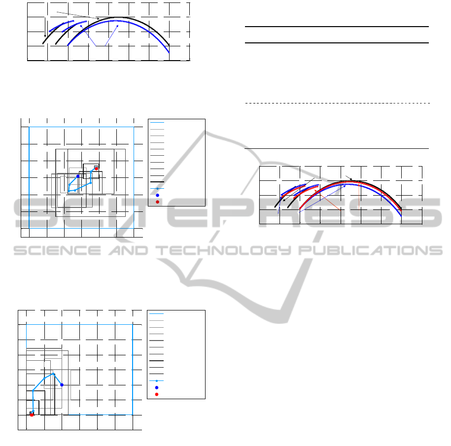
Figure 12: Initial and optimized shapes of the 2D F11

trawl-door. The flow direction is parallel to the x-axis.

Figure 13: Optimization history of the 2D F11 trawl-door

showing the lateral (x/c) and vertical (y/c) position of the

slats leading-edge.

Figure 14: Optimization history of the 2D F11 trawl-door

showing the inclination of the slats (



) and the flow angle

of attack (



5.2 3D Modern Trawl-Door

The 3D optimization is formulated in the same way

as the 2D one described in Section 5.2. However, the

minimum lift coefficient is now set as C

= 1.0. The

initial section shape is set as the optimum design

obtained in the 2D case. The span of the trawl-door

is set as 6.0 m and the aspect ratio is 2.4.

Table 2: Numerical results of the design optimization for

the 3D F11 trawl-door.

Variables Initial Optimized



x/c

0.0544 0.0600

y/c

0.0932 0.0732



[°]

20.00 20.00



[°]

2.69 0.69

1.00 1.00 0%

0.14 0.13

6%

7.52 7.55 +6%

Figure 15: Initial and optimized shapes of the 3D F11

trawl-door. The flow direction is parallel to the x-axis.

The numerical results of the 3D design

optimization are presented in Table 2. The 3D

optimum design, compared with the initial and

optimum 2D designs are presented in Fig. 15. The

results show that the values for the lift coefficient is

held constant while the drag coefficient is reduced

by 6% with the corresponding increase by 6% in the

lift-to-drag ratio. All the design variables are

adjusted slightly, aside from the slat inclination

angle, which is still at the lower bound.

5.3 2D Airfoil-Shaped Trawl-Door

The 2D airfoil-shaped trawl-door configuration is

shown in Fig. 2(b). The element shapes are kept

fixed. The main element has the shape of NACA

2412 and the leading-edge slat has the shape of

NACA 3210. The initial design configuration is: x/c

= 0.20, y/c = 0.08,



= 25°, and



= 8.59°. The

optimization problem is formulated the same way as

described in Section 5.1.

The numerical results of the design optimization

are presented in Table 3, and the initial and optimum

designs are illustrated in Fig. 16. The optimization

history with an illustration of the optimization path

as well as the vicinity size for each iteration, is

presented in Figs. 17 and 18.

The drag coefficient is reduced by 12% while

holding the lift coefficient constant. Again, the slat

inclination angle is near the lower bound.

-0.4 -0.2 0 0.2 0.4 0.6 0.8 1 1.2

-0.1

0.1

0.2

0.3

x/c

y/c

Initial

Optimized

-0.4 -0.3 -0.2 -0.1 0 0.1 0.2

-0.3

-0.2

-0.1

0.1

0.2

0.3

(x/c)

slats

(y/c)

slats

Design Space

Iteration 1

Iteration 2

Iteration 3

Iteration 4

Iteration 5

Iteration 6

Iteration 7

Iteration 8

Iteration 9

Optimization Path

Initial Design

Optimized Design

0 10 20 30 40 50 60



[°]



[°]

Design Space

Iteration 1

Iteration 2

Iteration 3

Iteration 4

Iteration 5

Iteration 6

Iteration 7

Iteration 8

Iteration 9

Optimization Path

Initial Design

Optimized Design

-0.4 -0.2 0 0.2 0.4 0.6 0.8 1 1.2

-0.1

0.1

0.2

0.3

x/c

y/c

2D initial

3D initial (2D opt.)

3D optimized

SIMULTECH2014-4thInternationalConferenceonSimulationandModelingMethodologies,Technologiesand

Applications

782

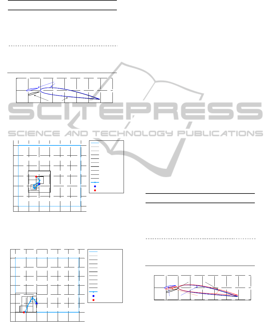
Table 3: Numerical results of the design optimization for

the 2D airfoil-shaped trawl-door.

Variables Initial Optimized



x/c

0.2000 0.2288

y/c

0.0800 0.0066



[°]

25.00 20.50



[°]

8.59 8.28

1.20 1.20 0%

0.020 0.017

12%

60.84 69.88 +12%

Figure 16: Initial and optimized shapes of the 2D airfoil-

shaped trawl-door. The flow direction is parallel to the x-

axis.

Figure 17: Optimization history of the 2D airfoil-shaped

trawl-door showing the lateral (x/c) and vertical (y/c)

position of the slats leading-edge.

Figure 18: Optimization history of the 2D airfoil-sahped

trawl-door showing the inclination of the slats (



) and the

flow angle of attack (



5.4 3D Airfoil-Shaped Trawl-Door

The 3D optimization task for the airfoil-shaped

trawl-door is formulated in the same way as the 3D

optimization of the F11 shape (described in Section

5.2). Table 4 shows the numerical results and Fig. 19

shows the initial and optimized designs.

The drag coefficient is reduced by 5% with the

corresponding increase by 6% in the lift-to-drag

ratio. There is a significant change is the shape from

2D to 3D indicating the importance of 3D flow

effects.

6 CONCLUSION

In this paper, a sequential approximate optimization

technique for hydrodynamic design of trawl-door

shapes has been presented. The design is based on

high-fidelity CFD simulation models. For the sake

of design cost reduction as well as reliability of the

optimization process, we utilize low-order

polynomial models and trust-region framework as a

convergence safeguard. Numerical studies are

carried out for both 2D and 3D cases with the final

designs obtained in a few iterations of the

optimization algorithm.

Table 4: Numerical results of the design optimization for

the 3D airfoil-shaped trawl-door.

Variables Initial Optimized



x/c

0.2288 0.0600

y/c

0.0066 0.0266



[°]

20.50 20.00



[°]

7.38 7.21

1.00 1.00 0%

0.050 0.047

5%

14.56 15.76 +6%

Figure 19: Initial and optimized shapes of the 3D airfoil-

shaped trawl-door. The flow direction is parallel to the x-

axis.

-0.4 -0.2 0 0.2 0.4 0.6 0.8 1 1.2

-0.2

0.2

x/c

y/c

Initial

Optimized

-0.4 -0.3 -0.2 -0.1 0 0.1 0.2

-0.3

-0.2

-0.1

0.1

0.2

0.3

(x/c)

slat

(y/c)

slat

Design Space

Iteration 1

Iteration 2

Iteration 3

Iteration 4

Iteration 5

Iteration 6

Iteration 7

Iteration 8

Iteration 9

Optimization Path

Initial Design

Optimized Design

0 10 20 30 40 50 60



[°]



[°]

Design Space

Iteration 1

Iteration 2

Iteration 3

Iteration 4

Iteration 5

Iteration 6

Iteration 7

Iteration 8

Iteration 9

Optimization Path

Initial Design

Optimized Design

-0.4 -0.2 0 0.2 0.4 0.6 0.8 1 1.2

-0.2

0.2

x/c

y/c

2D initial

3D initial (2D opt.) 3D optimized

Trawl-doorShapeOptimizationwith3DCFDModelsandLocalSurrogates

783

REFERENCES

FLUENT, ver. 14, ANSYS Inc., Southpointe, 275

Technology Drive, Canonsburg, PA 15317, 2012.

Garner, J., Botnvarpan og bunadur hennar, Fiskifelag

Islands, 1967.

Haraldsson, H.O., “Fluid Dynamics Simulation of Fishing

Gear,” M.Sc. Thesis, University of Iceland, May 1996,

ICEM CFD, ver. 14, ANSYS Inc., Southpointe, 275

Technology Drive, Canonsburg, PA 15317, 2012.

Jonsson, E., Leifsson, L., and Koziel, S. “Trawl-Door

Performance Analysis and Design Optimization with

CFD”, 2nd Int. Conf. on Simulation and Modeling

Methodologies, Technologies, and Applications

(SIMULTECH), Rome, Italy, July 28-31, 2012.

Jonsson, E., Hermannsson, E., Juliusson, M., Koziel, S.,

and Leifsson, L. “Computational Fluid Dynamic

Analysis and Shape Optimization of Trawl-Doors,”

51st AIAA Aerospace Sciences Meeting including the

New Horizons Forum and Aerospace Exposition,

Grapevine, Texas, January 7-10, 2013.

Ladson, C.L., “Effects of Independent Variation of Mach

and Reynolds Numbers on the Low-Speed

Aerodunamic Characteristics of the NACA 0012

airfoil Section,” NASA Technical Memorandum 4074,

NASA, 1988.

Leifsson, L., Koziel, S., Hermannsson, E., and Reza

Fakhraie, “Trawl-Door Design Optimization by Local

Surrogate Models,” 55th AIAA/ASMe/ASCE/AHS/SC

Structures, Structural Dynamics, and Materials

Conference, National Harbor, MD, January 2014.

Matlab, ver. R2014a, The Mathworks Inc., Natick,

Massachusetts, U.S.A, 2014.

Rumsey, C. L., Smith, B. R., and Huang, G. P.,

“Description of a Website Resource for Turbulence

Modeling Verification and Validation,” 40th AIAA

Fluid Dynamics Conference and Exhibit, AIAA Paper

2010-4742, Chicago, U.S.A., July 2010.

Tannehill, J.A., Anderson, D.A., and Pletcher, R.H.,

Computational fluid mechanics and heat transfer, 2nd

edition, Taylor & Francis, 1997.

Whicker, L. F., and Fehlner, L. F. “Free-Stream

Characteristics of a Family of Low-Aspect Ratio, All-

Movable Control Surfaces for Application to Ship

Design,” National Technical Information Service, U.S.

Department of Commerce, U.S.A, December 1958.

SIMULTECH2014-4thInternationalConferenceonSimulationandModelingMethodologies,Technologiesand

Applications

784