
Boosting of Neural Networks over MNIST Data
Eva Volna, Vaclav Kocian and Martin Kotyrba
Department of Informatics and computers, University of ostrava, 30 dubna 22, Ostrava, Czech Republic
Keywords: Boosting, Adaboost, MNIST Data, Pattern Recognition.
Abstract: The methods proposed in the article come out from a technique called boosting, which is based on the
principle of combining a large number of so-called weak classifiers into a strong classifier. The article is
focused on the possibility of increasing the efficiency of the algorithms via their appropriate combination,
and particularly increasing their reliability and reducing their time exigency. Time exigency does not mean
time exigency of the algorithm itself, nor its development, but time exigency of applying the algorithm to a
particular problem domain. Simulations and experiments of the proposed processes were performed in the
designed and created application environment. Experiments have been conducted over the MNIST database
of handwritten digits that is commonly used for training and testing in the field of machine learning. Finally,
a comparative experimental study with other approaches is presented. All achieved results are summarized
in a conclusion.
1 BOOSTING REVIEW
The two most popular methods for creating
ensembles are boosting (Schapire, 1999) and
bagging (Breiman, 1996). Boosting is reported to
give better results than bagging (Quinlan, 1996).
Both of them modify a set of training examples to
achieve diversity of weak learners in the ensemble.
As alternative methods we can mention
randomization based on a random modification of
base decision algorithm (Dietterich, 2000) or
Bayesian model averaging, which can even
outperform boosting in some cases (Davidson and
Fan, 2006). Boosting has its roots in a theoretical
framework for studying machine learning called the
‘PAC’ learning model, due to Valiant (Valiant,
1984). Schapire (Schapire, 1990) came up with the
first provable polynomial-time boosting algorithm in
1989. A year later, Freund (Freund, 1995) developed
a much more efficient boosting algorithm which,
although optimal in a certain sense, nevertheless
suffered from certain practical drawbacks. The first
experiments with these early boosting algorithms
were carried out by (Drucker, Schapire, and Simard,
1993) on an OCR task.
Boosting is a general method for improving the
accuracy of any given learning algorithm. The
algorithm takes as input the training set
,
,…,
,
where each
belongs to some
domain of the space , and each label
belongs to
some label set , where
∈
1,1
.
AdaBoost calls a given weak learning algorithm
repeatedly in a series of rounds 1,…,. One of
the main ideas of the algorithm is to maintain a
distribution of weights over the training set. The
weight of this distribution on -th training example
on round is denoted
. Initially, all weights are
set equally, but on each round, the weights of
incorrectly classified examples are increased so that
the weak learner is forced to focus on the hard
examples in the training set. The weak learner's job
is to find a weak hypothesis
:→1,1
appropriate for the distribution
. The goodness of
a weak hypothesis is measured by its error
(1):
:
(1)
Notice that the error
is measured with respect
to the distribution
on which the weak learner was
trained. In practice, the weak learner may be an
algorithm that can use the weights
on the training
examples. Alternatively, when this is not possible, a
subset of the training examples can be sampled
according to
, and these (unweighted) resampled
examples can be used to train the weak learner.
The most basic theoretical property of AdaBoost
concerns its ability to reduce the training error. Let
us write the error
of
as 0.5
. Since a
hypothesis that guesses each instance’s class at
random has an error rate of 0.5 (on binary
256
Volna E., Kocian V. and Kotyrba M..
Boosting of Neural Networks over MNIST Data.
DOI: 10.5220/0005131802560263
In Proceedings of the International Conference on Neural Computation Theory and Applications (NCTA-2014), pages 256-263
ISBN: 978-989-758-054-3
Copyright
c
2014 SCITEPRESS (Science and Technology Publications, Lda.)

problems),
thus measures how much better than
random are
’s predictions. Freund and Schapire
(Freund and Schapire, 1997) proved that the training
error (the fraction of mistakes on the training set) of
the final hypothesis is at most (2):
2
1
14
exp2
(2)
Thus, if each weak hypothesis is slightly better
than random so that
for some 0, then the
training error drops exponentially fast. However,
boosting algorithms required that such a lower
bound be known a priori before boosting begins.
In practice, knowledge of such a bound is very
difficult to obtain. AdaBoost, on the other hand, is
adaptive in that it adapts to the error rates of the
individual weak hypotheses. This is the basis of its
name ‘Ada’ is short for ‘adaptive’. (Freund and
Schapire, 1999).
2 ENSEMBLES OF CLASSIFIERS
The goal of ensemble learning methods is to
construct a collection (an ensemble) of individual
classifiers that are diverse and yet accurate. If it is
achieved, then highly accurate classification
decisions can be obtained by voting the decisions of
the individual classifiers in the ensemble.
We have proposed the method of learning on the
basis of the property of neural networks, which have
been noticed during another work (Kocian and
Volná, 2012), e.g. a major part of the adaptation is
performed during the first pass. We used neural
networks as generators of weak classifiers only, i.e.
such classifiers which are slightly better than a
random variable with uniform distribution. For weak
classifiers, their diversity is more important than
their accuracy. Therefore, it seemed appropriate to
use a greedy way in order to propose classifiers.
This approach uses only the power of the neural
network adaptation rule in the early stages of its
work and thus time is not lost due to a full
adaptation of the classifier.
2.1 Performance and Diversity
The most significant experimental part of the article
focused on dealing with text (machine readable) in
particular. However, we were not limited to printed
text. The experiment has been conducted over the
MNIST database (LeCun et al., 2014). The MNIST
database is a large database of handwritten digits
that is commonly used for training and testing in the
field of machine learning.
We have proposed several approaches to
improve performance of boosting (Iwakura et al.,
2010). In our experiment, we try to increase
diversity of classifiers by the following methods. It
specifically relates to such innovations concerning
training sets.
Filtering of inputs;
Randomly changing the order of the training
examples;
Doubling occurrences of incorrectly classified
examples in a training set;
All these neural networks used the algorithm
for an elimination of irrelevant inputs as
proposed in (Kocian et al., 2011).
2.1.1 Proposed Neural-Networks-based
Classifiers
In consequent text, we have used the following
nomenclature refers to neural networks:
– input value;
– required (expected) output value;
– input of neuron y;
– output of neuron y;
– learning parameter;
– formula for calculating a neuron output
value (activation function) y
out
= φ(y
in
);
∆ – formula for calculating a change of a
weight value.
We have used a total of five types of neural
networks in the study. We have used codes N1-N4
for single-layer networks, and N5 for a two-layer
network. The proposed ensembles of neural-
networks-based classifiers are basically a set of m
classifiers. All the m classifiers work with the same
set of n inputs. Each of the m classifiers tries to learn
to recognize objects of one class in the input patterns
of size n. Details about the parameters of the
networks are shown in Table 1. All the neural
networks used the winner-takes-all strategy for
output neurons (Y
1
,.....,Y
n
) when they worked in the
active mode. So only one output neuron with the
highest
value could be active. The Y
i
is
considered the winner if and only if ∀:
⋁
⋀, i.e. the winner is the neuron
with the highest output value
. In the case that
more neurons have the same output value, the
winner is considered the first one in the order. Since
Adaline did not perform well with the basic learning
rule
(Fausett, 1994), we assume that the
BoostingofNeuralNetworksoverMNISTData
257
cause lays in the relatively big number of patterns
and inputs and therefore possibly the big value of
. That is, why we have normalized value of
by the sigmoid function.
Table 1: Parameters of classifiers.
Type
(x)
Δ
N1
Modified Adaline Rule
N2
1
1exp
Delta Rule
N3
Hebb Rule
N4
Perceptron Rule
N5
1
1exp
Back Propagation Rule
The classifier is an alias for an instance of a
neural network. Each classifier was created
separately and adapted by only one pass through the
training set. After that the test set was presented and
all achieved results were recorded in detail:
Lists of correctly and incorrectly classified
patterns;
Time of adaptation.
Ensemble is a set of 100 classifiers, i.e. 100
instances of neural networks. Each ensemble is
defined by two parameters in total:
The base algorithms, i.e. what types of neural
networks form the ensemble (Table 1);
Configuring of rising the diversity - i.e. what
methods were used to increase the diversity in
the process of creation of classifiers for the
ensemble. We used three methods, Filtering,
Shuffling and Doubling.
Similarly to the classifier, the ensemble was also
re-created. All achieved results were recorded in
detail. Achieved parameters that were recorded for
ensembles:
Patterns that were correctly identified by all
classifiers;
Patterns that were incorrectly recognized by
all classifier;
Maximal, minimal and average error of
classifiers over the training set;
Maximal, minimal and average error of
classifiers over the test set.
2.1.2 Diversity Enhancement Configuration
This section describes the method to increase the
diversity of classifiers that were used in the proposal
of a specific ensemble. We used 6 bases of
algorithms in total: N1 represents Adaline, N2
represents delta rule, N3 represents Hebbian
network, N4 represents perceptron, N5 represents
Back Propagation network and the sixth base N1-N5
represents all ensembles contain 20 specific
instances of a specific type. In the test, each
combination of three methods was tested on 50
ensembles that were composed from classifiers
formed over a given base of algorithms. Figure 1
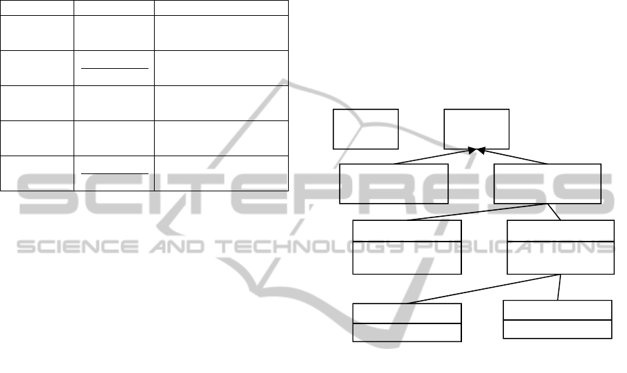
shows briefly the logical structure of the experiment.
Figure 1: Logical structure of the experiment. Each base of
algorithm has been tested with 12 different diversity
enhancing configurations. Total of 50 ensembles has been
created over each base of algorithm and diversity
enhancing configuration. Each ensemble consisted of 100
classifiers.
Classifiers were generated as instances of N1-
N5. The accuracy of each generated classifier was
verified on both the test and the training set. The
results achieved by each classifier were stored in a
database and evaluated at the end of the experiment.
For purpose of our experiment we have defined an
ensemble as a group of 100 classifiers generated
over the same set of algorithms with the same
configuration of the generator. One set of ensembles
has been made over all available algorithms. Twelve
different configurations have been tested within each
set. Each configuration was tested 50 times in every
set of ensembles. Therefore there have been created
and tested 61250100360000 different
instances of neural networks.
Figure 2 represents a creation of one classifier
instance through a generator. It utilized the available
library of algorithms, training set and configuration.
Configuration specifies presentation of the training
Base of
algorithms 1
Base of
algorithms 6
…
Diversity enhancing
configuration 1
Diversity enhancing
configuration 12
…
Ensemble 1
Base of algorithms
Enhancing config.
Ensemble 50
Base of algorithms
Enhancing config.
…
Classifier 1
Network type
…
Classifier 100
Network type
NCTA2014-InternationalConferenceonNeuralComputationTheoryandApplications
258
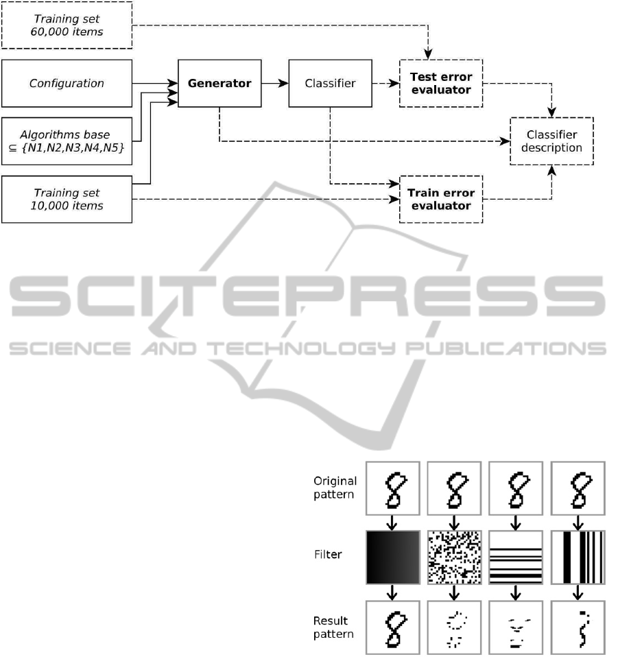
Figure 2: Block diagram of classifier generation. Dashed parts apply only to the experiment. In the real system, the
procedure final product would be the classifier itself.
set. In the next step (indicated by dashed line) each
generated classifier was subjected to the test of
accuracy on both the training and the test set. At the
end of the whole procedure, we had obtained
complete information about all correctly and
incorrectly classified patterns, about base algorithm
and about the configuration. The experiment was
conducted over the data from the MNIST database
(LeCun et al., 2014). The training set contains 60000
patterns and the test set contains 10000 patterns.
Patterns are stored in the database as a 28x28 pixel
images with 256 grayscale. As the examples
represent digits, it is obvious, that they can be
divided into 10 classes, therefore all tested neural
networks had a total of 10 output neurons. The
highest number of input neurons was2828784.
2.2 Methods of Classifiers Diversity
Enhancing
We propose the input filters as a method for
enhancing diversity of classifiers. The main idea of
input filter is, that classifier ‘sees’ only a part of the
input. It forces the classifier to focus its attention
only on certain features (parts of pattern). It should
increase the diversity of individual classifiers
generated. Input filter is represented by a bitmap F
of the same size as the original pattern. The
classifier ‘sees’ the input pattern ‘through’ matrix F
while only bits of F, which have value of 1 are
‘transparent’. The blank filter is represented by a
matrix whose pixels are all set to value of 1.
Topology of classifier always reflects the current
filter in the sense that the number of input neurons is
equal to the number of bits with value of 1 in the
bitmap F. It implies that the topology of classifiers,
when using a non-blank filter, is smaller and less
demanding in terms of memory space and CPU time.
Figure 3 shows the example of application of
different filters to the pattern representing the
number ‘8’. We have used the following three
modes of the input filters:
Blank;
Random (white noise);
Random Streak. In this mode, vertical or
horizontal filter was picked-up with the same
probability of 0.5.
Figure 3: Example of use of different filters on the input
pattern with the image number ‘8’. In the top row we can
see four different filter matrices, in the bottom row there
are the results of the filtration (what the classifier can see).
Through the blank filter (left) the original shape of the
pattern is visible. Displayed filters from the left: The blank
filter, the random filter, the horizontal streak filter, the
vertical streak filter.
Shuffling. Training patterns were presented in
random order. This can force the classifier to go the
other path during the learning.
BoostingofNeuralNetworksoverMNISTData
259

Doubling. Patterns that were correctly identified
by all tested classifiers in the ensemble, were
removed from the training set. Patterns that have not
been properly learned by any classifier in the
ensemble, were included twice in the training set.
We have used the diversity of classifiers in the
ensembles as the criterion for judging the success of
algorithms and configurations. Moreover, we have
focused mainly on performance at the test set of
patterns. We have expressed the diversity as the
reciprocal of the count of patterns, which were not
correctly classified by any of the classifiers in the
ensemble. The smaller number of unrecognized
patterns means the more successful ensemble. If the
diversity on the testing set was remarkably worse
than the diversity on the training set, we have
experienced over-fitting. The results of the
experiments are summarized in Tables 2-4. The
tables share a common column marking:
TAvg – average percentage of unrecognized
patterns in the training set;
GAvg –average percentage of unrecognized
patterns in the test set
GAvg/TAvg error ratio. Generalization
capabilities. The higher value indicates the
higher overfitting. So the smaller number
means the higher quality of the classifier.
Table 2: Achieved experimental results.
Type TAvg GAvg GAvg/TAvg
N1 0.760 1.093 1.438
N2 0.610 0.943 1.545
N3 0.900 1.423 1.581
N4 0.770 1.093 1.419
N5 0.360 0.510 1.416
N1-N5 0.430 0.630 1.465
In Table 2 we can see that the average
performance of the Back Propagation network (N5)
is the best. It also shares the best GAvg/TAvg value
with the perceptron (N4). On the other side, the
Hebb (N3) is the worst, it gives the worst
performance on both the average error and the
GAvg/TAvg value.
Table 3: Comparison of quality of ensembles by doubling
and shuffling.
Doubling Shuffling
Yes No Yes No
TAvg 0.348 0.928 0.540 0.737
GAvg 0.718 1.180 0.833 1.066
GAvg/TAvg 2.063 1.271 1.542 1.446
Looking at Table 3, the doubling method affects
parameters of generated ensembles. The doubling
enhances diversity, but it also significantly reduces
the ensemble’s generalization capabilities. It was
expected as the doubling forces the classifiers to
focus on the particular portion of the train set.
Concerning shuffling, it slightly enhances diversity
and reduces the generalization capabilities. The
shuffling is weaker than the doubling but we cannot,
if it is better or worse than the shuffling.
Table 4: Comparison of quality of ensembles by filters.
Filter TAvg GAvg GAvg/TAvg
Streak 0.288 0.378 1.312
Random 0.570 0.824 1.445
Blank 1.058 1.644 1.553
In Table 4 we can investigate the influence of
different filters on the ensembles behaviour. It is
clear from the values in the table that the filtering is
the right way to go through. The filtering method put
the ensemble’s performance forward in both the
average error and the generalization capabilities. We
can also see that the streak filter performs
significantly better than the random one.
3 BOOSTING OF NEURAL
NETWORKS
In the section we have used two different types of
neural networks. Hebb network and Back
Propagation network. Details about initial
configurations of the used networks are shown in
Table 5. Both neural networks used the winner-
takes-all strategy for output neurons when worked in
the active mode. Just as in our previous work
(Kocian and Volná, 2012), we have used a slightly
modified Hebb rule with identity activation function
y
out
= y
in
. This simple modification allows using the
winner-takes-all strategy without losing information
about the input to the neuron. Back Propagation
network was adapted using the sloppy adaptation as
we have proposed in (Kocian and Volná, 2012).
Table 5: Neural networks initial configuration.
Type
(x)
Δ
Hebb
∙∙; 1
BP
2
1exp
1
∙
1
2
1
1
0.04
We worked with the following approaches to
patterns weights: the lowest weight of a pattern
(e.g. weight of the pattern that was recognized by all
weak classifiers from an ensemble) was recorded in
each iteration. When designing the training set, there
NCTA2014-InternationalConferenceonNeuralComputationTheoryandApplications
260
were patterns with a weight value d inserted into the
training set
1 times. It means that patterns
with the lowest weight value were eliminated from
the training set, the others were inserted into the
training set repeatedly by the size of their weight
values. The order of patterns in the training set was
chosen randomly. In the process, the training set was
gradually enlarged. The training set was able to
reach its size of 10
, which significantly slowed its
adaptation. To reduce enormous ‘puffing’ of the
training set, we tried to substitute multiple insertions
with dynamic manipulation with a learning rate. In
this way, the neural networks set specific learning
rate
(3) for each i-th pattern and each t-th
iteration.
1
(3)
It turned out that neural networks did not work
properly with such a modified algorithm. Handling
the learning rate corresponds to the multiple
insertion of a pattern in the same place in the
training set. Neural networks are adapted well if
patterns are uniformly spread in the training set.
Therefore, it was necessary to follow multiple
insertion of patterns so that the training set could
always mix before its use. Methods of enhanced
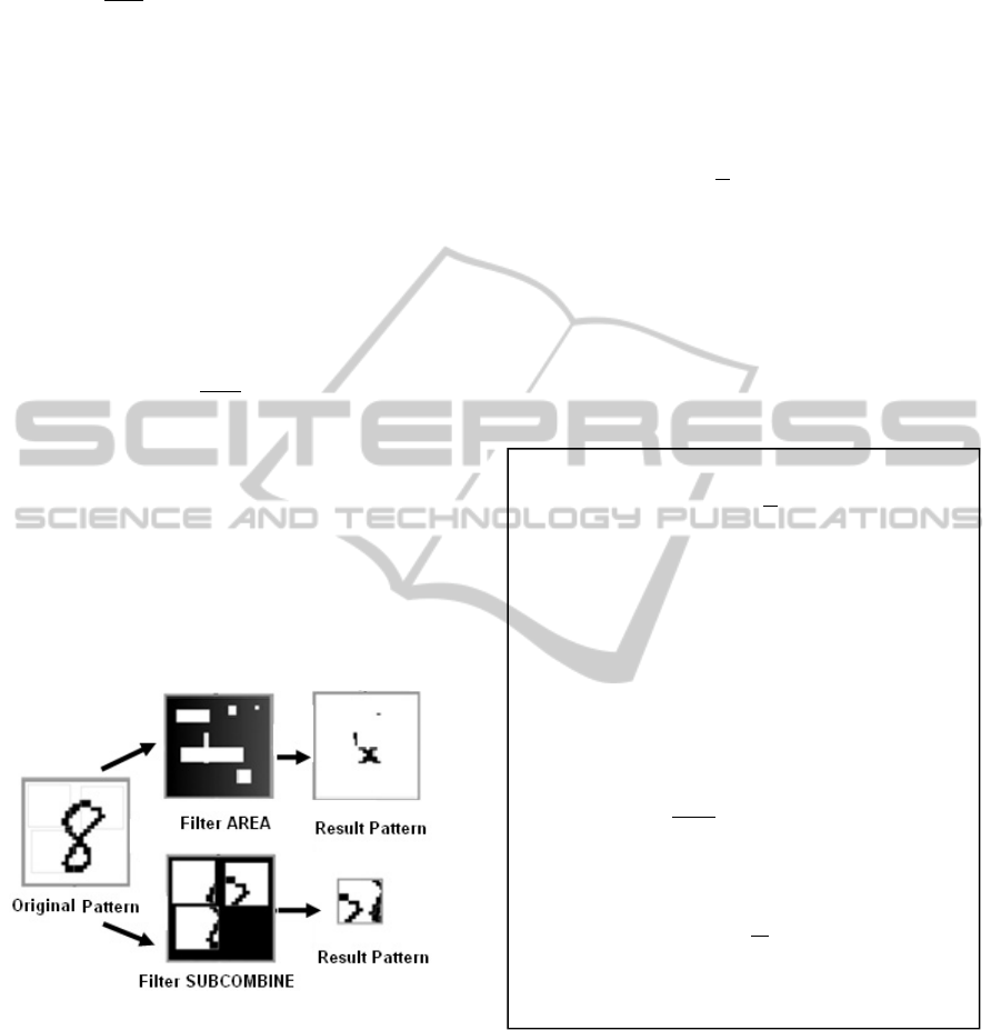
filtering were shown in Figure 4.
Figure 4: Filters AREA and SUBCOMBINE.
The method ‘subareas’ is a generalization of the
strip filter. Filter AREA was always defined by six
rectangular ‘holes’ in the mask through which the
neural network saw input vectors. Size and location
of rectangles were chosen randomly.
Procedural filter SUBCOMBINE transforms the
original pattern S to the working pattern S so that
from the original pattern randomly selects a few
square areas of random identical size p x m and all
of these areas are combined into one pattern.
The idea of the type of a filter is the fact that some
parts of selected areas are overlapped.
We have proposed several approaches to
improve performance of boosting algorithm
AdaBoost.M1 based on (Freund and Schapire, 1996)
that are defined as follows. Given set of examples
〈
,
,…,
,
〉
with labels
∈
1,…,
. The initial distribution is set uniformly
over , so
for all . To compute
distribution
from
,
and the last weak
hypothesis, we multiply the weight of example i by:
Some number ∈0,1 if
classifies
correctly ( example’s weight goes down);
‘1’ otherwise (example’s weight stays
unchanged).
The weights are then renormalized by dividing
by the normalization constant
. The whole
boosting algorithm is shown in Figure 5.
Figure 5: boosting algorithm AdaBoost.M1.
Exactly as we have expected, the more classifiers
was in the ensemble, the more difficult it was to find
another sufficient classifier which satisfies the
condition
. This difficulty tended to grow
exponentially fast and together with the growing
training set it made the adaptation process very slow.
The experiment results are shown in Table 6,
where BP8 means Back Propagation network with 8
hidden neurons and BP50 with 50 hidden neurons.
,
1,
max
∈
log
1
:
begin
Initialize:
for all ;
1;
Repeat
Repeat
Generate a weak classifier
;
Learn
with
;
get its hypothesis
:→;
Calculate
according to (1);
Until
Calculate
/1
;
Calculate
∑
;
Update the weight distribution:
Increment ;
Until end condition;
The final hypothesis is:
End.
BoostingofNeuralNetworksoverMNISTData
261
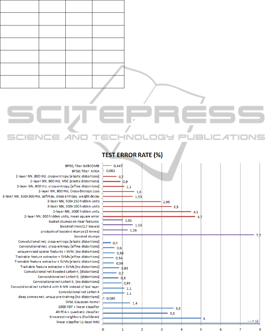
Table 6: Boosting results.
Classifier;
FILTER
Test
Err.
Train
Err.
Train
Size
Hebb;
AREA
10.907 10.860 226444
Hebb;
SUBCOMB
8.190 8.820 316168
BP8;
AREA
6.503 7.010 698539
BP8;
SUBCOMB
6.720 7.400 647553
BP50;
AREA
0.062 2.890 38513603
BP50;
SUBCOMB
0.447 4.090 12543975
4 RESULTS AND COMPARISON
WITH OTHER METHODS
Many methods have been tested with the MNIST
database of handwritten digits (LeCun et al., 2014).
While recognising digits is only one of many
problems involved in designing a practical
recognition system, it is an excellent benchmark for
comparing shape recognition methods. Though
many existing method combine a hand-crafted
feature extractor and a training classifier, the
comparable study concentrates on adaptive methods
that operate directly on size-normalized images.
A comparison of our approach with other
methods is shown in Figure 6. The graph represents
the achieved test of several methods over MNIST
database. Here, GREEN colour represents our
results (Table 6), RED colour represents results of
multilayer neural networks, VIOLET colour
represents results of busted methods, and BLUE
colour represents other results. It means the
following methods: a linear classifier, K-nearest-
neighbors, a quadratic classifier, RBF, SVM, a deep
convex net, convolutional nets and various
combinations of these methods. Details about these
methods are given in (LeCun et al., 1998).
Figure 6: Test error over MNIST database of handwritten digits. Comparison with other methods: GREEN colour
represents our results, RED colour represents results of multilayer neural networks, VIOLET colour represents results of
busted methods, and BLUE colour represents other results.
NCTA2014-InternationalConferenceonNeuralComputationTheoryandApplications
262

5 CONCLUSIONS
We have tested five types of neural networks and
three different methods of diversity enhancement.
We have proposed the one-cycle learning method for
neural networks, same as the method of diversity
enhancement which we call input filtering. Based on
the experimental study results we can formulate the
following outcomes:
Neural networks in general look suitable as
the base algorithms for classifiers ensembles.
The method of one-cycle learning looks
suitable for ensembles building too.
Filtering gave surprisingly good results as the
method of diversity enhancement.
Doubling of patterns gave surprisingly well
results too. We expected that this method
would lead to over-fitting, but this assumption
did not prove correct.
We expected more from shuffling of patterns.
But as the results show, doubling of patterns is
more permissible.
Boosting results are shown in Table 6 looking at it,
we can pronounce the following:
The best performance (train error 0.062%, test
error 2.89%) has been reached with the Back
Propagation network with 50 hidden neurons.
The worst performance has been reached with
the Hebbian network.
Green colour represents our results in Figure
6, which are promising by comparison with
other approaches.
Adaboost, neural networks and input filters look
as a very promising combination. Although we have
used only random filters, the performance of the
combined classifier was satisfactory. We have
proved the positive influence of input filters.
Nevertheless the random method of input filters
selecting makes the adaptation process very time
consuming. We have to look for more sophisticated
methods of detecting problematic areas in the
patterns. Once such areas are found, we will able to
design and possibly generalize some method of the
bespoke input filter construction.
ACKNOWLEDGEMENTS
The research steps described here have been
financially supported by the University of Ostrava
grant SGS16/PrF/2014.
REFERENCES
Breiman, L. (1996). Bagging predictors. In Machine
Learning. (pp. 123-140).
Davidson, I., and Fan, W. (2006). When efficient model
averaging out-performs boosting and bagging.
Knowledge Discovery in Databases, 478-486.
Dietterich, T. G. (2000). An experimental comparison of
three methods for constructing ensembles of decision
trees: Bagging, boosting, and randomization. Machine
learning, 139-157.
Drucker, H., Schapire, R., and Simard, P. (1993). Boosting
performance in neural networks. Int. Journ. of Pattern
Recognition. and Artificial Intelligence, 705-719.
Fausett, L. V. (1994). Fundamentals of Neural Networks.
Englewood Cliffs, New Jersey: Prentice-Hall, Inc.
Freund, Y. (1995). Boosting a weak learning algorithm by
majority. Information and Computation, 256-285.
Freund, Y., and Schapire, R. (1996). Experiments with a
New Boosting Algorithm. ICML, 148-156.
Freund, Y., and Schapire, R. E. (1997). A decision-
theoretic generalization of on-line learning and an
application to boosting. J. of Comp. and System
Sciences, 119–139.
Freund, Y., and Schapire, R. (1999). A short introduction
to boosting. J. Japan. Soc. for Artif. Intel., 771-780.
Iwakura, T., Okamoto, S., and Asakawa, K. (2010). An
AdaBoost Using a Weak-Learner Generating Several
Weak-Hypotheses for Large Training Data of Natural
Language Processing. IEEJ Transactions on
Electronics, Information and Systems, 83-91.
Kocian, V., Volná, E., Janošek, M., and Kotyrba, M.
(2011). Optimizatinon of training sets for Hebbian-
learningbased classifiers. In Proc. of the 17th Int.
Conf. on Soft Computing, Mendel 2011, pp. 185-190.
Kocian, V., and Volná, E. (2012). Ensembles of neural-
networks-based classifiers. In Proc. of the 18th Int.
Conf. on Soft Computing, Mendel 2012, pp. 256-261.
LeCun, Y. Bottou, L. Bengio, Y. and Haffner, P. (1998)
Gradient-based learning applied to document
recognition. Proceedings of the IEEE, 86(11):2278-
2324, November.
LeCun, Y., Cortes, C., and Burges, C. (2014). Te MNIST
Database. Retrieved from http://yann.lecun.com/
exdb/mnist/
Quinlan, J. R. (1996). Bagging, boosting, and C4.5.
Thirteenth National Conference on Artificial
Intelligence, (pp. 725-730).
Schapire, R. E. (1990). The strength of weak learnability.
Machine Learning, 197-227.
Schapire, R. E. (1999). A brief introduction to boosting.
Sixteenth International Joint Conference on Artificial
Intelligence IJCAI (pp. 1401–1406). Morgan
Kaufmann Publishers Inc.
Valiant, L. G. (1984). A theory of the learnable.
Communications of the ACM, 1134-1142.
BoostingofNeuralNetworksoverMNISTData
263
