
Traveling Salesman Problem Solutions by Using Passive
Neural Networks
Andrzej Luksza and Wieslaw Sienko
Department of Electrical Engineering, Gdynia Maritime University,
Morska 81-86, Gdynia, Poland
Abstract. Presented in this paper numeric experiments on random, relative
large travelling salesman problems, show that the passive neural networks can
be used as an efficient, dynamic optimization tool for combinatorial
programming. Moreover, the passive neural networks, when implemented in
VLSI technology, could be a basis for structure of bio-inspired processors, for
real-time optimizations.
1 Introduction
Optimization programming and in particular combinatorial optimization, is an
essential tool for engineering design. It is well known that a standard for
combinatorial optimization is Traveling Salesman Problem (TSP), classified as
NP-hard.
Methods of TSP solving could be divided into two groups. The first group
consists of algorithmic methods, among which special attention is given to heuristic
algorithms – as evolutionary (EA) and ant. The second group is based on the energy
minimization principle. In that group of methods special attention is focused on
Hopfield neural networks, whose second use – beside implementations of
autoassociative memories – are optimization tasks. According to our knowledge
Hopfield neural networks have not been commercially implemented as physical
objects, being primarily a mathematical model. A physical implementation of the
energy minimization system is so-called “commercial quantum computer” − D-Wave.
Currently the available D-Wave computers are able to solve TSP for 6 cities [1].
The purpose of this paper is to point out how passive neural networks used as
energy minimizers set up a new structure for combinatorial optimization problems
solving. Using the model of the passive neural network as an energy minimizer is not
new [2]. The considerations presented in this paper are modified version of the above
mentioned research and can be seen as a justification for current search for power
efficient processors with computational efficiency unattainable by traditional
computers.
2 D-Wave Quantum Computers – Energy Minimizer
It seemed that the quantum computer concept, due to physical principles and
Luksza A. and Sienko W..
Traveling Salesman Problem Solutions by Using Passive Neural Networks.
DOI: 10.5220/0005132800690077
In Proceedings of the International Workshop on Artificial Neural Networks and Intelligent Information Processing (ANNIIP-2014), pages 69-77
ISBN: 978-989-758-041-3
Copyright
c
2014 SCITEPRESS (Science and Technology Publications, Lda.)

technological limitations, would remain only a theoretical model. No ability of
quantum computers implementation was claimed by one of the leading physicists in
the following [3] “No quantum computer can ever be built that can outperform a
classical computer if the latter would have its components and processing speed
scaled to Planck units”.
The general premise for such a statement is unavoidable presence of decoherence
phenomena for temperature T > 0. Meanwhile, past few years the concept of quantum
computers has been turned into a physical system, which is nowadays known as the
D-Wave system. Such a system, regardless of doubts to its truly quantum nature is
currently available on the market. The basic property of the D-Wave system is
optimization problems solving which can be defined as Ising-like objective function.
Thus the D-wave system, treated as a physical network of coupled qubits, solves
optimization problems by achieving the state of minimum energy. The introductory
description of the numerical experiments done by D-Wave computers can be found in
[1] paper.
3 Ising’s Models
Ising’s models are known in statistical mechanics as a simplified description of
ferromagnetism. One considers system of N nodes with the assigned values +1 or –1
(spin-up or spin-down, respectively) to the spin variables s
i
, i = 1,…, N. The set of
numbers {s
i
} determines a configuration of the entire system and its energy as
follows:
ji
N
i
ijiijiI
sBsssH
,1
}{
,
(1)
where <i, j> is a pair of the closest neighboring spins, <i, j> = <j, i>, B is an external
magnetic field (energy constant) and
ij
is the interaction energy.
In the case of the D-Wave computer, its quantum processor is created by the
coupled qubits network, so the Hamiltonian of such a network is given as follows:
),(1
}{
ji
N
i
iijiijiI
shssJsH
,
(2)
where (i,j) are pairs of coupled qubits, S
i
is an initial state of the i-th qubit (0 or 1), J
ij
is an interaction energy and h
i
is i-th qubit bias energy.
By so called adiabatic quantum annealing, the network is aiming at the energy
minimum described by J
ij
and h
i
constants. It is easy to find out, that the minimum of
the objective function for such a model is given as
),(1
min
ji
N
i
iijiij
shssJ
.
(3)
Hence all the optimization problems, for which formulas (2) and (3) could be used,
are implementable by D-Wave computer.
70

Thus, TSP optimization problem given by the objective function and constraints as
n
i
ijij
yd
1
min
,
(4)
..
1
,
1,…,,
1
, 1,…,,
∈
0,1
, ,
(5)
(6)
can be transformed into the form of the D-Wave Hamiltonian (2). The constants d
ij
denote the known distances between cities. The variable y
ij
is equal to 1 when a
salesman moves directly from the city i to the city j, otherwise it is equal to 0. The
objective function (4) achieves the minimum value for all n-cycles representing the
salesman routes. The constraint (6) means that the i-th city occurs only once on the
salesman path. The constraint (5) excludes a possibility of simultaneous occurrence of
two or more cities at j-th position in n-cycle.
The standard formulation of optimization programming for the objective function
(4) subject to the constraints (5) and (6), is to create appropriate Lagrange function,
i.e. obtained by summing objective function and the penalties function with the
appropriate weights.
The Hamiltonian, given by formula (2) can be obtained by implementation of the
stable dynamic system, whose elements (e.g. qubits) are related to the interactions
matrix {J
ij
}. Thus the matrix {J
ij
} is a square symmetric matrix, whose non-diagonal
elements describe qubits interaction energy and diagonal elements describe qubits
own energy. It is easy to note, that in case of TSP, the interaction matrix consists of
distances d
ij
, modified by constraints. This type of matrix has been proposed by
Hopfield and Tank, where interaction matrix takes the form of the weight matrix
(connections) between neurons with step activation functions {0,1} [4].
4 TSP Solutions obtained by Using Passive Neural Networks
A passive n-neuron network is a dynamic system, described by the state-space
equation [5]
,
(7)
where x = [x
1
,…,x
n
]
T
is a state vector, W is a weight matrix, θ(x) = [θ(x
1
), …, θ(x
n
)]
T
is a neuron activation functions vector, I
B
is a bias vector of the network, d is an input
data vector,
0
> 0 – integrator losses. Activation functions are passive, fulfilling
condition μ
1
≤ θ(x
i
) / x
i
≤ μ
1
; μ
1
, μ
1
∈
0,∞
. In particular, activation functions could
be unity step functions.
A special feature of such a neural network is the following weight matrix
sa
WWW
,
(8)
71

where W
a
is an antisymmetric component, W
s
is a symmetric component and
∈.
The primary usage of the passive neural network is an associative memory
implementation
,
,…,
,
(9)
where vectors m
i
for i = 1,…,k are points of equilibrium. The essence of such an
implementation is the following learning mechanism:
1. for
= 0 (equation (8)) network weight matrix is antisymmetric. Vectors m
i
(equation (9)) are becoming isolated points of equilibrium.
2. for
≠ 0 the symmetric component W
s
secures the compensation of the
network losses and as a result one obtains the state bifurcations to equilibrium points
∈. This means that the selected
are becoming the centres of attraction.
The above learning mechanism refers to genetic mechanisms such as
recombination – antisymmetric component, and selection – symmetric component.
It is worth noting that the key problem of this paper can be formulated, as follows:
By application of passive neural networks with the connection matrix (8), it is
possible to separate the realization of the objective function (4) and constraints (5)
and (6). Hence the formulation of TSP solution by the passive neural network
structure is as follows:
Given n cities localizations and distances d
ij
between cities, then in Eq.(4)
variables
∈
0,1
,,1,…, describe i-th city at j-th position in n cycle,
respectively. Assigning to each city, neural subnetwork containing n output neurons
with activation step functions
∙
∈
0,1
and denoting neurons outputs
∙
≡
, ,1,…,, one obtains the following statement 1.
Statement 1. Given memory matrix M, where dim M = [(n+2) × n]:
10⋯⋯0
010⋯0
⋮0⋱⋱⋮
⋮⋮⋱10
00⋯01
11⋯11
11⋯11
(10)
then it can be implemented by using a lossless (ω
0
= 0), autonomous (d = 0) neural
subnetwork with weight matrix W
i
[(n + 2) × (n + 2)]
0⋯0
⋮⋱⋮ ⋮ ⋮
0⋯0
⋯
0
⋯
∆
2
,
0,1,…,,∆0,
(11)
under conditions of a bias vector, as follows:
0,0…0,
,
∆
.
(12)
Indeed
∙
, where
∈.
72

It is easy to notice that only one of the outputs
ij
(·) of the output neurons can be
in the high state (+1).
Statement 2. By compatible connections of n-subnets described in statement 1,
one obtains a neural network consisting of n
2
– output neurons and 2n – hidden
neurons. The main property of such a network is a high state (+1) of only one neuron
in a group of n-neurons representing the i-th city. Hence, such a network fulfils the
constraint (6) for TSP.
It should be noted that the same mechanism of generation of the vectors {0,1} can
also be used to enforce a high state (+1) at the output of any group of neurons. Thus,
it is possible to implement the constraints (5) for TSP, too. Since for the physical
network
0
> 0 in Eq.(7), the lossy term must be compensated for. Hence one obtains:
Statement 3. The autonomous neural network (i.e. d ≡ 0 in equation (7)),
described by the state-space equation
,
(13)
where W
n
is the weight matrix [(n
2
+4n) × (n
2
+4n)], structured accordingly to
statement 1 and statement 2, I
B
is the bias vector, γ
i
> 0 is compensation of network
losses,
0
– integrator losses,
is a generator of vectors {0,1}, fulfilling constraints (5) and (6) of the TSP
optimization problem.
For n = 2 the structure of the weight matrix W
n
is as follows:
0000
00
00
0000
0000
000000
00
000000
00
000
000000
00
∆000000
00
000
0000
00
00
∆0000
0
000000
00
0
00000
∆ 0 0
0
0
0000000
0
0
000000
∆
__________
0,0,0,0,,∆,,∆,,∆,,∆
,
where B = w
1
− w
0
> 0, > 0.
Matrix W
n
retains the structure of W
2
for any n (n – number of cities).
Note 1
It should be noted that neural network described in statement 3 is lossless with
equilibria, given by vectors {0,1} fulfilling TSP constraints, and with coexisting limit
cycles.
As mentioned above, the Hamiltonian given by equation (2) can be obtained by
implementation of the stable dynamic system. Hence for TSP the square symmetric
matrix W
s
={[d
ij
]}, i, j = 1,…,n is formed wherein elements describe interactions
energy of the output neurons.
Submatrices [d
ij
] are (n×n) blocks of the matrix W
s
, wherein [d
ii
] = [0]. The
matrix W
s
contains n
2
of such submatrices. Hence one obtains:
Statement 4. The autonomous neural network described by the state-space
equation
73

,
(14)
where W
s0
is a symmetric matrix containing matrix W
s
supplemented by zeroes
elements to the dimension [(n
2
+ 4n) × (n
2
+ 4n)] (remaining components of equation
(14) are the same as in equation (13)), is asymptotically stable for < 0.
Global equilibrium point of such a network is determined by the minimum of the
energy dissipated by the network.
An example of the W
s0
matrix structure, for three cities (n = 3) is as follows:
0000
0
000
0
0
000
0
0
0
0000
0
000
0
0000
0
0
0
000
0
0
000
0
0000
for n = 3, dimW
s0
= (9 + 12) × (9 + 12).
Statement 5. According to the Note1, the total energy E(t), t > 0, dissipated in the
network is given as follows:
,
(15)
where E(t) is the energy of output neurons interactions and
< 0.
Since dE / dt < 0, the system described by equation (14) is asymptotically stable.
The minimum of energy E(t) is determined by
min
min
,
,
,
(16)
which means that the minimum of the objective function for TSP has been reached.
5 Example of the TSP Solution
In further research of the network properties, TSP for n = 30 cities was verified. The
cities location is presented in Fig. 1.
For solving above issue of the TSP, a network model described by equations (13) and
(14), with the following parameters, has been used:
100
∙
1000,
(17)
where W
n
0,
,
,∆
,
7,
14, ∆5.25,
0.625for1,…,
,
1.5for
1,…,
4, 1,
W
s0
is the matrix of distances between cities, wherein cities are deployed at square
with an edge length equal to 1.
74
a) b)
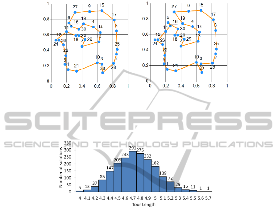
Fig. 1. TSP test cities map with a) the optimal path, b) the shortest found path,
const.
The number of all possible routes is equal to 29! / 2 = 4.4 × 10
30
. The optimal
solution seems to be the path shown in Fig. 1a, the length of which is 3.89. During the
experiment of the above thousand tests, a number of correct paths were found. Fig. 2
shows a histogram of the found path lengths.
Fig. 2. Histogram of path lengths found by the neural network: average length = 4.75, standard
deviation = 0.26, min = 3.98, max = 5.67.
The shortest found path – length 3.98 – is shown in Fig. 1b. This path is longer by 2%
in comparison to the optimal solution (Fig. 1a). The path from Fig. 1b can be
improved by the city inversions of 3 pairs of cities (6, 16), (12, 24) and (3, 23). Such
city inversion on the path can be detected and corrected by implementation of a
simple algorithm.
The results were compared to the results described by Hopfield and Tank [4]
where the shortest found path length was 15% longer than the optimal route.
According to the histogram shown in Fig. 2 the TSP solution found by the passive
neural network are feasible and stable – non feasible solutions are unstable and not
observable. The number of local equilibria depends on the value of parameter
.
Hence, it is worth noting that there exists a possibility to minimize the number of
local equilibria by the procedure of variable values for
. Thus, starting the state of the
neural network from
i
≤ 0, i = 1,…, n
2
+ 4n and stepwise increasing these values
during integration, one obtains feasible solutions with fewer number of local
equilibria. The histogram of the found path lengths for the cities map from Fig.1 is
75
shown in Fig. 3.
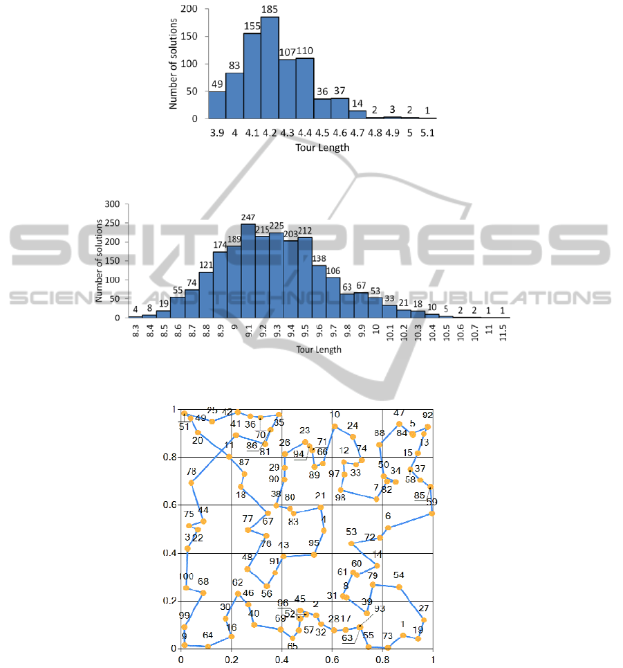
Fig.3. Histogram of path lengths found with increasing : average length = 4.34, standard
deviation = 0.26, min = 3.89.
Fig. 4. Histogram of path lengths found with increasing for 100 cities: average length = 9.29,
standard deviation = 0.40, min = 8.30.
Fig. 5. The shortest found path for 100 cities, length = 8.30.
It should be noted, that similar mechanism for optimization of Hopfield neural
networks was used by Abe and Gee [6].
76

Using the above mentioned variable
mechanism, the passive neural network
finds also feasible solutions of the TSP for n > 100 cities, in a few minutes of
integrations (on a standard PC). The histogram of feasible TSP solutions for n = 100
cities and an example of solution are shown in Fig. 4 and Fig. 5, respectively.
It is easy to notice that the path from Fig. 5 can be improved by the city
inversions, namely (78, 11) into (78, 20) and (11, 20) into (11, 41).
6 Conclusions
Presented in this paper numeric experiments on random, relative large travelling
salesman problems, show that the passive neural networks can be used as an efficient,
dynamic optimization tool for combinatorial programming. Moreover, the passive
neural network, when implemented in VLSI technology could be a basis for structure
of bio-inspired processor, for real-time optimization. Contrary to the sceptical opinion
on physical implementation of Hopfield-type neural networks [7,8], we claim that the
passive neural networks are implementable in VLSI technology as very large scale
networks and applicable as analogue processors to solve in real time some
challenging problems.
References
1. Warren, R. H.: Numeric Experiments on the Commercial Quantum Computer, Notices of
the AMS, Vol. 60, No 11 (2013)
2. Luksza, A.: Badanie Realizowalności Wielkich Sieci Neuronowych, Dissertation (in
Polish), Gdańsk University of Technology (1997)
3. t’Hooft, G.: Determinism and Dissipation in Quantum Gravity, arXiv:hep-th/0003005 v
2,16 (2000)
4. Hopfield, J. J., Tank, D. W.: Neural computation of decisions in optimization problems,
Biological Cybernatics, vol.52 (1985)
5. Sienko, W., Luksza, A., Citko, W.: On Properties of Passive Neural Networks,
Wydawnictwa Uczelniane WSM, Gdynia (1993), ISSN – 0324 – 8887
6. Abe, S., Gee, A. H.: Global Convergence of the Hopfield Neural Network with Nonzero
Diagonal Elements, IEEE Tr. on CAS, vol.42, No 1 (1995)
7. Gee, A. H., Prager, R.W.: Limitations of Neural Networks for Solving Traveling Salesman
Problems, IEEE Tr. on Neural Networks, vol.6, No 1 (1995)
8. Haykin, S.: Neural Networks and Learning Machines, Person Education, Inc., N.J. (2009)
77
