
Consensus Coordination in the Network of
Autonomous Intersection Management
Chairit Wuthishuwong and Ansgar Traechtler
Heinz Nixdorf Institute, Control Engineering and Mechatronics Department,
University Paderborn, Fuestenallee, Paderborn, Germany
Keywords: Autonomous Intersection Management, Intelligent Transportation System, Autonomous Vehicle, Vehicle to
Infrastructure Communication, Infrastructure to Infrastructure Communication, Consensus Algorithm.
Abstract: The Autonomous Intersection Management (AIM) will be a future method for the Intelligent Transportation
System. It combines wireless communication and the autonomous vehicle in order to create the new concept
for managing road traffic more safely and efficienly. The distributed control principle is applied to the
intersection network to control the traffic in the macroscopic level. The Vehicle to Infrastructure (V2I) and
Infrastructure to Infrastructure (I2I) communication are used to exchange the traffic information between a
single autonomous vehicle to the network of autonomous intersections The discrete time consensus
algorithm is implemented to coordinate the gross traffic density of an intersection and its neighborhoods in
the network. The boundary condition for the uncongested flow is created by using the Greenshield’s traffic
model. The proposed method represents the ability to maintain the traffic flow rate of each intersection and
operates with the uncongested flow condition. The simulation results of the network of a multiple
autonomous intersection are provided.
1 INTRODUCTION
The traffic congestion problem is increasingly
becoming a severe problem in the road
transportation. The research in the Intelligent
Transportation System tries to find a solution to
improve the traffic safety and efficiency. There were
several researches in controlling the traffic signal
due to the fixed timing traffic signal, indicating a
poor performance in managing traffic. One of the
active solutions is using the technique of the
adaptive traffic signalling. The traffic signal can be
adjusted adaptively based on the current traffic
situation. There are many methods to adjust the
traffic signal. The commercial solution called
SCOOT (Robertson, 1991) determines the period of
green and red light by using the queue length of each
street. In (Chiu, 1993), Fuzzy logic was applied to
update the signal, based on the constructing rules.
The Autonomous Intersection Management
(AIM) concept is a totally autonomous system that
combines the technology of the autonomous vehicle
and the wireless communication. According to the
intelligence of an autonomous vehicle
(Wuthishuwong, 2008), the road accidents that are
caused by human driver errors can be reduced. The
objectives of creating a full autonomous system are
to improve the traffic safety and traffic efficiency by
using autonomous vehicles and an autonomous
intersection manager. The AIM (Dresner, 2008) was
studied based on the multi-agents technique. Vehicle
agents communicate to an intersection agent to
reserve the area. The successful reservation will
have no confliction with the others. Otherwise, the
reservation will be rejected. In (Naumann, 1998),
(Zou, 2003) used the same concept but without the
intersection agent. Vehicle agent negotiates with
each other in order to cross an intersection. In
(Wuthishuwong, 2013) used the V2I communication
to plan the safe trajectory for each vehicle whilst
crossing an intersection. The extend version from a
single AIM to the multiple AIM in (Wuthishuwong,
2013) was studied the technique for maintaining the
traffic flow in the network by coordinating the local
traffic information between its neighbourhood.
In this paper, the authors propose the consensus
algorithm in order to coordinate the traffic
information between each autonomous intersection
in the network. The multiple intersections scenario is
modelled As well, the communication topology
794
Wuthishuwong C. and Traechtler A..
Consensus Coordination in the Network of Autonomous Intersection Management.
DOI: 10.5220/0005148607940801
In Proceedings of the 11th International Conference on Informatics in Control, Automation and Robotics (IVC&ITS-2014), pages 794-801
ISBN: 978-989-758-040-6
Copyright
c
2014 SCITEPRESS (Science and Technology Publications, Lda.)
between Vehicle to Infrastructure (V2I) and
Infrastructure to Infrastructure (I2I) are designed.
Maintaining the continuity of the traffic flow in the
network, the boundary condition of the uncongested
flow is derived based on the Greenshield’s traffic
model. The simulation of a multiple Autonomous
Intersection Management is presented. The results
are plotted and evaluated with the Greenshield’s
model
2 INTERSECTION NETWORK
The intersection network is modelled by connecting
9 single intersections, where each intersection has 4
ways. It is based on the distributed control structure.
Then, a single intersection is considered as an
autonomous agent that has ability to control itself,
whilst the control strategy is dependent on the
information between its neighborhoods.
The graph theory (Murray, 2009) is used to
visualize and interpret the interaction of a network.
Technically, each intersection manager is assigned
by a node and the connection between each node is
represented by an edge. However, there are 2 classes
of a node relationship.
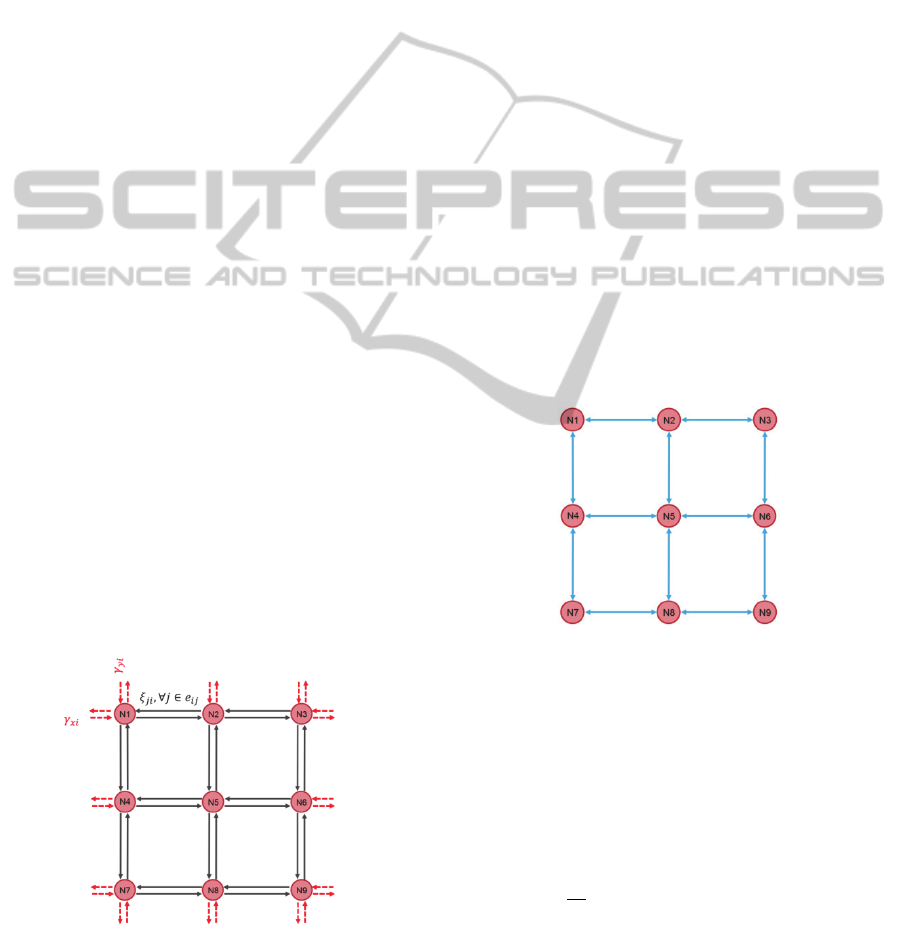
2.1 Street Network
The street network is modeled based on the real
physical connection of each intersection. Typically,
an intersection is connected through an incoming
and outgoing street. Hence, the street network is a
set of street that connects a group of neighbored
intersections as illustrated in Fig.1. At the street
network, a single intersection acts as a central
manager. Each single intersection collects the local
traffic density on the connected street by counting
Figure 1: Network of streets with the direction flow of all
intersection.
the requested messages that are transmitted from the
incoming vehicles over the V2I communication.
Therefore, each intersection manager in the network
is identical and it responds to manage only its own
local intersection. The collected traffic density
information of each intersection can be determined
by summing the traffic density of all incoming
streets to intersection.
∈
,
,∈
(1)
Where,
is the gross incoming traffic density of the
intersection,
is the incoming traffic density of a
street has traveled from intersection to intersection
, and
,
is the external incoming traffic from the
sources , connect to the intersection .
2.2 Communication Network
The communication topology of the intersection
network is illustrated in Fig. 2. The connection
between couple of nodes uses the bi-directional
communication. Each node, which represents an
intersection manager, can either receive or transmit
the data package to their destination node
Figure 2: Intersection communication network topology.
The properties of a graph theory are used to
represent the relationship of the intersection
network. The adjacency element
, will have value
1 when there is an edge between each node,
otherwise the value is equal to 0.
1,
,
∈
0,
;,
∈
(2)
The degree matrix describes the number of
connections at each intersection.
ConsensusCoordinationintheNetworkofAutonomousIntersectionManagement
795

,
,
0,
;,
∈
(3)
The Laplacian matrix describes the complete
relationship of the intersection network. The simple
way to determine the Laplacian matrix is subtracting
the degree matrix with the adjacency matrix.
(4)
Where; is the row element of the matrix, is the
column element of the matrix,
is the adjacency
matrix,
is the degree matrix, and is the
Laplacian matrix.
3 CONSENSUS COORDINATION
OF AIM
In this work, the discrete consensus algorithm is
implemented for coordinating the traffic information
in AIM in order to balance the overall traffic flow in
the network. The consensus algorithm has been
recently studied in robot application such as robot
formation in (Ren, 2007; Olfati-Saber, 2003; Olfati-
Saber, 2007). Naturally, it is the distributed control
that gives the convergence property, which fits for
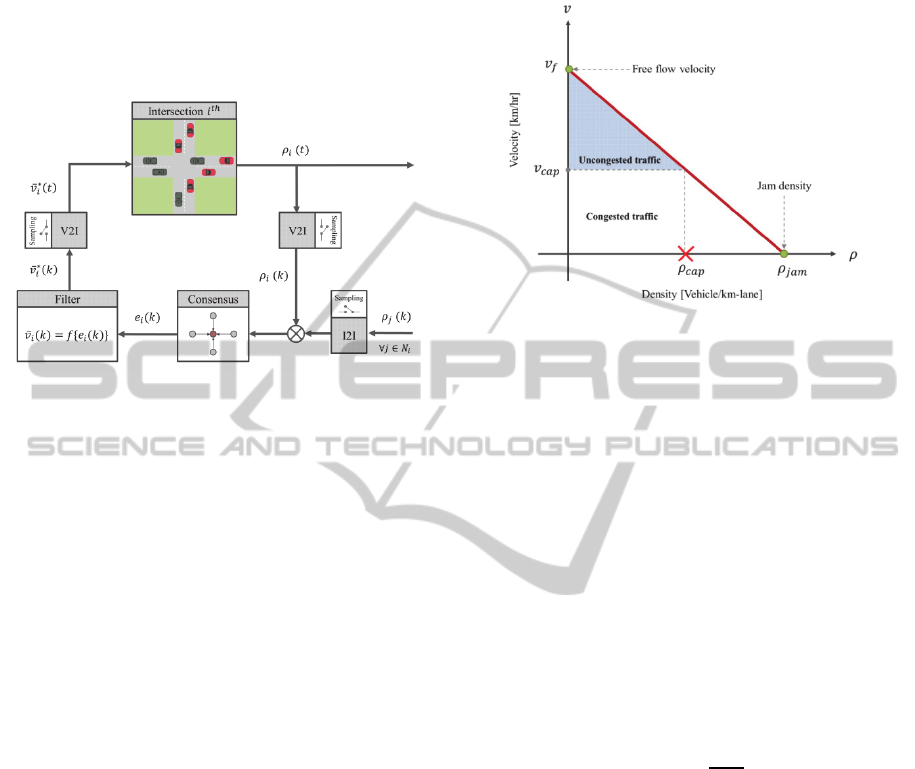
the large scale system. The system architecture of
the multiple, autonomous intersections management
is illustrated in Fig. 3.
Figure 3: The system architecture of the multiple
autonomous intersections management.
Each intersection acts as the centralized
controller. The traffic density of each intersection is
collected in the street network layer by using V2I
communication and this information is distributed to
its neighborhoods in the intersection network layer
over I2I communication. The AIM will compute the
control command, based on the traffic density of
itself and its neighborhoods.
The consensus algorithm is applied to coordinate
the traffic information among the intersections in the
group. The traffic density is used as the coordinated
information, as well as, representing the state of an
intersection. The dynamics of each local intersection
and a global network can be expressed as the
following equation.
∈
(5)
(6)
Substituting the gross traffic density of each
intersection, which is defined in Eq.1, the consensus
of a collective AIM can be derived as:
⋮
∙
⋮
∙
⋮
(7)
The discrete time consensus is derived by applying
the difference equation. Then, the discrete time
consensus for a local intersection and a global
network can be expressed as the following equation.
1
∈
(8)
1
(9)
Where, is a Perron matrix and is the
step size 0. The sufficient conditions for the
stability of a consensus in the network are provided
in [9].
The control system of a mulitple autonomous
intersections is composed of nine units of AIM,
which is the distributed control schema. Thus, each
intersection control strategy is identical. The closed
loop control block diagram of the autonomous traffic
control of a single intersection is illustrated in Fig.4.
The autonomous vehicle is used in AIM system
and practically AIM can only prioritze the timing of
crossing an intersection. Thus, the control variable is
the incoming time which can be transformed to the
average velocity when the distance between a
vehicle and intersection is known. Basically, every
vehicle has to send the requesting message to AIM
before crossing an intersection. With this point, the
ICINCO2014-11thInternationalConferenceonInformaticsinControl,AutomationandRobotics
796
traffic density and number of vehicles approaching
an intersection, is measured through the V2I
communication. It counts the number of messages of
the incoming vehicles and substracts the number of
outgoing vehicles. However, the information is in a
discrete time domain after sampling.
Figure 4: Closed loop control block diagram of a single
intersection.
In order to control the traffic flow of an
intersection, the traffic density of the neighborhoods
is inputted through I2I communication. The
consensus algorithm coordinates the information
from itself with its neighborhood in order to
determine the desired value of the traffic density
following the Eq. 9. Therefore, the error term of
each intersection is the difference between the
desired traffic density and the current traffic density
value. It can be expressed as the following equation.
1
(10)
Technically, the consensus algorithm try to
balance the traffic density between the local
intersections. This means it will maintain the level of
traffic density closed to its neighborhoods, to keep
the low variation between them. Theoretically, the
error term must be minimized and approach zero in
the finite time in order to make the current traffic
density equal to the desired traffic density.
Refering to the field of transportation engineer, the
traffic model is composed of three corresponding
parameters: traffic density, traffic flow rate and
average velocity. These relationships are used to
represent the macroscopic traffic. In this work, the
Greenshield’s model is used as the reference traffic
model. For controlling the traffic, the condition of
the congested and uncongested traffic are defined by
using the empirical data of the traffic density,
average velocity and traffic flow rate. the
relationship between the average velocity and the
traffic density with the boundary of congested and
uncongested traffic is illustrated in Fig.5.
Figure 5: Greenshield’s traffic model: the relationship
between the average velocity and the traffic density.
According to the parameters of the Greenshield’s
model (Hall, 1996), the free flow velocity
is
given at 91 km/hr and the jamming density
is
given at 78 vehicles/km/lane. The velocity at
capacity
is given at 46 km/hr. The velocity at
capacity is the lower boundary of the average
velocity that vehicles can drive under the
uncongested traffic. The traffic will begin to congest
after this boundary, if the vehicles cannot keep the
driving velocity at least at this level. Consequently,
the traffic density at capacity
is the maximum
number of vehicles on the street that still keeps the
average velocity within the boundary. It can be
determined as:
1
(11)
The traffic density at capacity is round up to 38
vehicles/km/lane. The boundary condition of the
uncongested traffic can be summarized into the
following equations.
0
(12)
The uncongested traffic is satisfied when the average
velocity is higher than the velocity at capacity and
less than the free flow velocity, as well as, the traffic
density being greater than zero and less than the
traffic density at capacity. On the other hand, the
congested traffic conditions are vice versa.
The second relationship represents the relationship
between the traffic flow rate and the traffic density.
ConsensusCoordinationintheNetworkofAutonomousIntersectionManagement
797
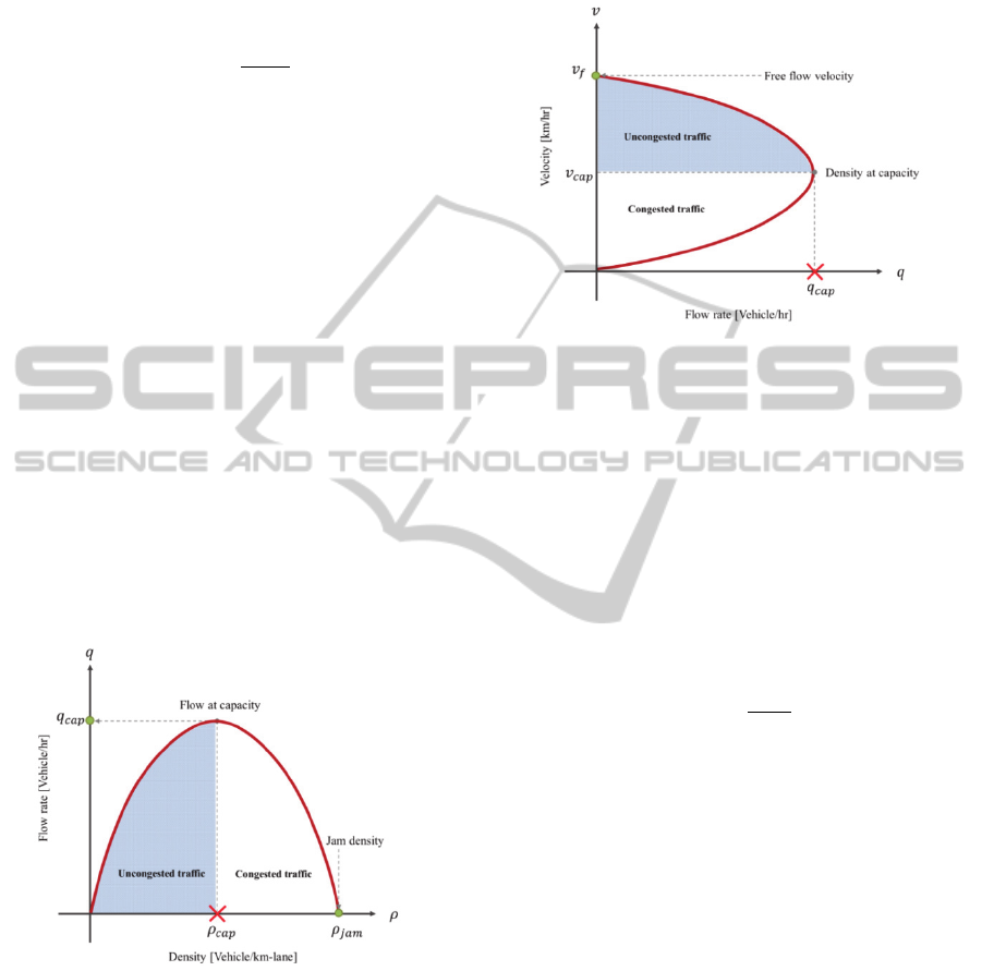
The relationship between these two parameters is
defined by a parabolic function. With the provided
parameters, the traffic flow at capacity
can be
determined as:
(13)
The traffic flow rate at the capacity will be
approximately 1,800 vehicles/hr. It can be said that
the boundary of the uncongested traffic is 0
. However, this boundary condition cannot be
alone used to indicate the traffic situation. The
uncongested traffic and congested traffic condition
share the same boundary since the relationship is the
parabolic function. The traffic flow of the
uncongested traffic is in the left region of the graph
and the derivative gives the positive value. That
means the average velocity is increasing from zero
until it reaches the boundary of the traffic flow at
capacity. Meanwhile, the traffic flow under the
congested traffic is on the other side with the
negative slope. The flow rate is gradually decreased
to zero after the point of traffic flow at capacity is
reached. The Greenshield’s model of the relationship
between the traffic flow rate and the traffic density
with the boundary of congested and uncongested
traffic is illustrated in Fig.6.
Figure 6: Greenshield’s traffic model: the relationship
between the traffic flow rate and the traffic density.
The Greenshield’s model of the relationship between
the average velocity and the traffic flow rate with the
boundary of congested and uncongested traffic is
illustrated in the Fig. 7. The uncongested traffic is
represented in the upper part of the graph. On the
contrary, the lower part of the graph represents the
congested traffic condition. In addition, the graph
shows that at the equilibrium point, the average
velocity at capacity and the traffic flow rate at
capacity provides the value of the traffic density at
capacity.
Figure 7: Greenshield’s traffic model: the relationship
between the average velocity and the traffic flow rate.
With the Greenshield’s traffic model, the traffic of
an intersection is controllable. In order to manage
the current traffic density to meet the desired traffic
density, the Greenshield’s relationship of an average
velocity and a traffic density is implemented. Since
the model gives the direct relationship between
them, it is obvious that changing an average velocity
is the way to minimize the traffic density error of an
intersection. The average velocity in the discrete
time can be derived as:
̅
̅
1
(14)
In the control block diagram, the filter is
implemented for smoothing the output response in
order to remove the short term fluctuation. The
technique of the moving average is applied by
weighting the value between the current computed
value with the previous desired value. The weighting
coefficient is called the degree of filtering and the
summation of them will be unity. It is called the
exponential moving average filter. Technically, the
function of this filter is identical to the first order
low pass filter in the electronics circuit, suppressing
the amplitude of a signal so that the frequency is
higher than the cut-off frequency. The exponential
moving average filter for the desired average
velocity can be expressed as:
̅
∗
̅
1
̅
∗
1
(15)
Where, ̅
∗
is the desired average velocity for an
intersection at time step , ̅
is the computed
ICINCO2014-11thInternationalConferenceonInformaticsinControl,AutomationandRobotics
798
average velocity from the Greenshield’s model at
time step , ̅
∗
1 is the previous time step
1 of a desired average velocity and is the
weight coefficient, ∈
0,1
.
Since, the intersection network is designed,
based on the distributed control, every intersection
control structure is identical as presented in Fig. 4.
For this reason, the collective of all sub systems,
intersection manager, represents the characteristic of
the intersection network. The closed loop control
block diagram of the intersection network can be
illustrated in Fig.8.
Figure 8: Closed loop control block diagram of the
intersection network.
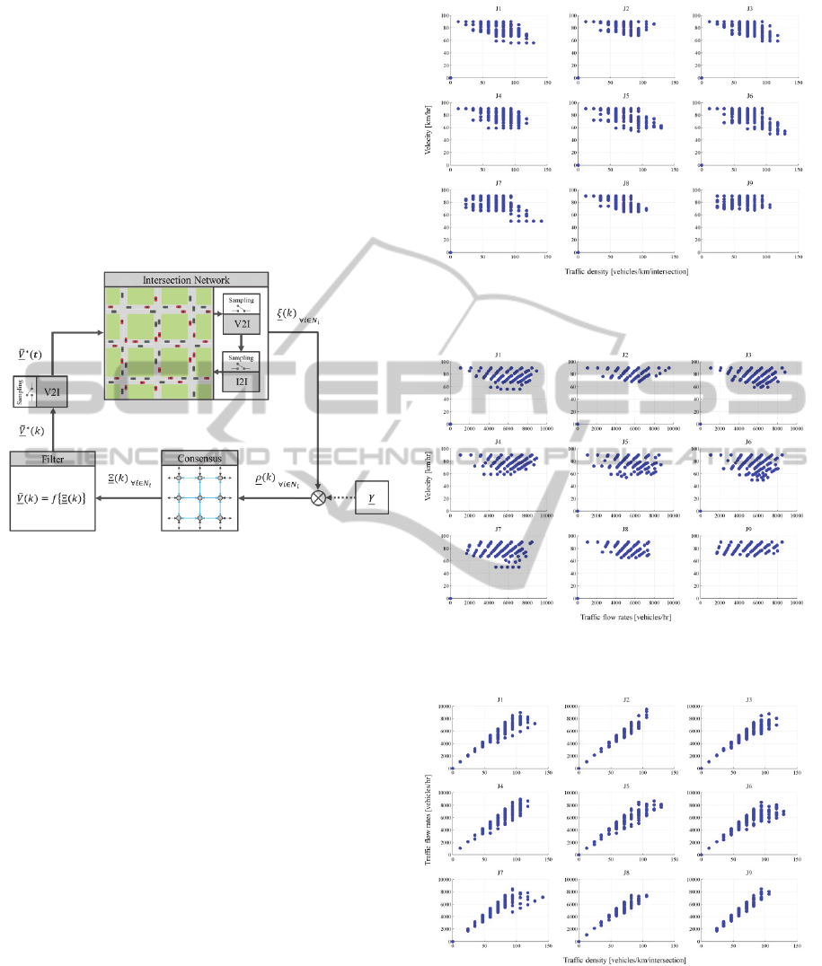
4 SIMULATION RESULTS
The simulation results of the multiple autonomous
intersection management, which were implemented,
based on the consensus algorithm with the
Greenshield’s traffic model, is presented. The
inputted traffic flow rate of all 12 sources is assigned
randomly. The range of the traffic flow rate is set
between 1,000-2,000 vehicles/hr.
All vehicles generate their own route randomly. The
results of the relationship between 3 traffic
parameters of each intersection are plotted. The
paired relationship between average velocity, traffic
density and traffic flow rate is shown in Fig. 9, 10,
and 11 respectively. In addition, the collecting plots
of all intersections, compared to the Greenshield’s
model are shown in Fig12, 13 and 14 respectively.
The corresponding plot of all traffic parameters of 9
intersections is shown in Fig.15.
Figure 9: The average velocity and the traffic density
relationship of each intersection in the network.
Figure 10: The average velocity and the traffic flow rate
relationship of each intersection in the network.
Figure 11: The traffic flow rate and the traffic density
relationship of each intersection in the network.
ConsensusCoordinationintheNetworkofAutonomousIntersectionManagement
799
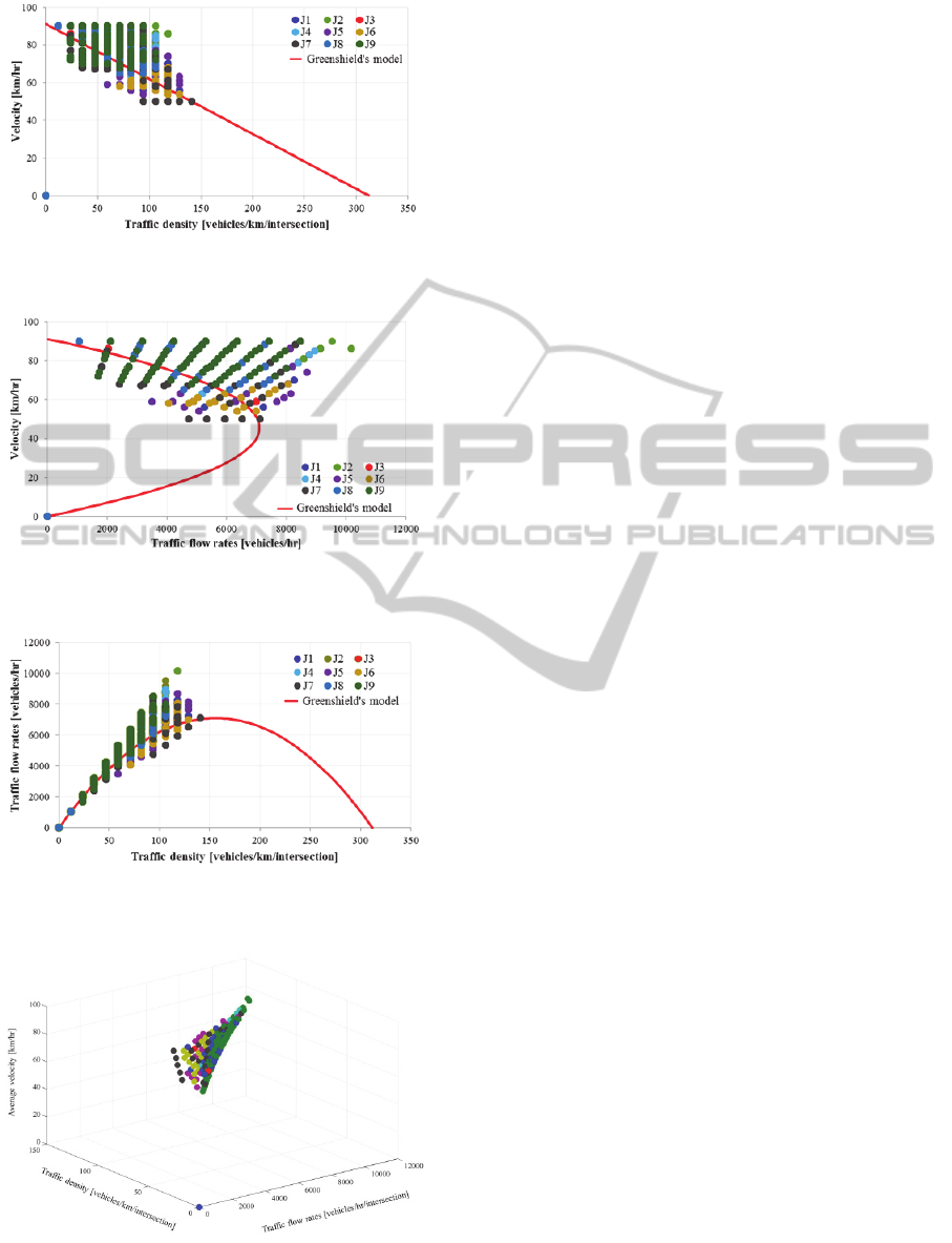
Figure 12: Collecting plot of the average velocity and the
traffic density, compared with the Greenshield’s model.
Figure 13: Collecting plot of the average velocity and the
traffic flow rate, compared with the Greenshield’s model.
Figure 14: Collecting plot of the traffic flow rate and the
traffic density, compared with the Greenshield’s model.
Figure 15: Summary plot of all traffic parameters, traffic
flow rate, traffic density and average velocity of 9
intersections.
The results show all intersections can maintain the
level of traffic density, average velocity and the
traffic flow rate, within the uncongested condition.
As well, AIM provides better efficiency in traffic
flow rates, compared to the theoretical value that
given by Greenshield’s model.
5 CONCLUSIONS
This work introduces the coordination method for
multiple, autonomous intersections by using discrete
consensus algorithm with the Greenshield’s model.
In this paper, the proposed method presents the
success performance in managing the traffic in the
network of multiple autonomous intersections. The
simulation results show every intersection in the
network can operate under the uncongested flow
condition and provides a contribution in traffic flow
rate capability. The attached video presents the
success driving under the green wave concept that
all vehicles can maintain continuous driving and
crossing multiple intersections without stop.
ACKNOWLEDGEMENTS
This research is funded by Ministry of Innovation,
Science, Research, and Technology of the Federal
State North-Rhine-Westphalia, Germany through the
International Graduate School (IGS) of Dynamic
Intelligent System. This research work is the
continued project of the Autonomous Intersection
Management under the supervision of Prof. Ansgar
Traechtler, Heinz Nixdorf Institute, Control
engineering and Mechatronics department,
University of Paderborn.
REFERENCES
Robertson, Dennis, I. & Bretherton, David. R. 1991,
‘Optimizing networks of traffic signals in real-time-
The SCOOT method’, In IEEE Transactions on
Vehicular Technology, Vol. 40.
Chiu, Stephen & Chand, Sujeet 1993, ‘Adaptive traffic
signal control using fuzzy logic’, In IEEE Conference
on Fuzzy Systems, San Francisco, CA, USA, pp. 1371-
1376.
Wuthishuwong, C, Silawatchananai, C. & Panichkun, M.
2008, ‘Navigation and control of an intelligent vehicle
by using stand-alone GPS, compass and laser range
finder’, In IEEE International Conference on Robotics
and Biomimetics.
ICINCO2014-11thInternationalConferenceonInformaticsinControl,AutomationandRobotics
800

Dresner, Kurt & Stone, Peter 2008, ‘A multiagent
approach to autonomous intersection management’, In
Journal of Artificial Intelligent Research, pp.591-656.
Naumann, Rolf, Rasche, Rainer & Tacken, Jürgen 1998,
‘Managing autonomous vehicles at intersections’, In
IEEE Intelligent Systems, pp. 82-86.
Zou, Xi. & Levinson, David 2003, ‘Vehicle based
intersection management with intelligent agents’, In
ITS America Annual meeting Proceedings.
Wuthishuwong, C. & Traechtler, A. 2013, ‘Vehicle to
Infrastructure based safe trajectory planning for
Autonomous Intersection Management’, In 13
th
IEEE
International Conference on ITS Telecommunication,
Tampere, Finland.
Wuthishuwong, C. & Traechtler, A. 2013, ‘Coordination
of multiple autonomous intersections by using local
neighborhood information’, In 2
nd
IEEE International
Conference on Connected Vehicles and Expo, Las
Vegas, USA.
Wuthishuwong, C. Traechtler, A. 2014 ‘Stability of the
consensus in the network of multiple autonomous
intersection management’, In 20
th
IEEE International
Conference on Automation and Computing.
Ren, Wei, Beard, Randal. W. & Atkins, Ella. M. 2007,
‘Information consensus in multivehicle cooperative
control’, In IEEE Control systems magazine.
Olfati-Saber, Reza & Murray, Richard M. 2003,
‘Consensus protocols for networkes of dynamic
agents’, In Proceedings of the 2003 American Control
Conference, vol.2, pp. 951-956.
Olfati-Saber, Reza Fax, J. Alex Murray, Richard M. 2007,
‘Consensus and cooperation in networked multi-agent
system’, In Proceedings of the IEEE, pp. 215-233.
Murray, Richard M. 2009, ‘Introduction to Graph Theory
and Consensus’, In Lecture notes, Caltech Control and
Dynamical Systems.
Hall, Fred. L. 1996, ‘Traffic stream characteristics’, In
Federal High Way Administration (FHWA) research
publication, U.S. DOT.
ConsensusCoordinationintheNetworkofAutonomousIntersectionManagement
801
