
Smooth Trajectory Generation with 4D Space Analysis for Dynamic
Obstacle Avoidance
Suhyeon Gim
1,2
, Lounis Adouane
1
, Sukhan Lee
2
and Jean-Pierre Derutin
1
1
Institut Pascal/Universit´e Blaise Pascal UMR6602, 63177, Aubi´ere Cedex, France
2
SungKyunKwan University, Seoburo 2066, 440-746, Suwon, Korea
Keywords:
Continuous Curvature Path, Dynamic Obstacle Avoidance, Velocity Planning.
Abstract:
This paper presents smooth trajectory generation scheme for obstacle avoidance in static and dynamic en-
vironment. The smooth trajectory has successive two steps where smooth path is generated firstly and then
corresponding velocity is planned along the path. Smooth path of continuous curvature is composed by para-
metrically adjusted clothoids with proposed algorithm and then the safe velocity planning is carried out in the
4D configuration framework. Two circles are used to completely surround the used nonholonomic car-like
vehicle, this permit to check the probable future vehicle’s collisions and to have space-time analysis. Some
demonstrative simulations show the strong potential of the proposed smooth and flexible methodology for
future experimentations with actual vehicles.
1 INTRODUCTION
Autonomous navigated vehicle or semi-autonomous
driver assistant system has been attracting a lot of
robotics research and industry fields for more than a
decade. One of the most important issues is trajec-
tory generation or path planning capability to manage
a safe motion in a variety of risky environments. In
path planning scheme, there are two kinds of planners
(or planning algorithm) which are characterized either
by global or local (Solea and Nunes, 2006), (Villa-
gra et al., 2012). The global path planner gives a
general navigational information (the path/trajectory
to follow) to the vehicle to go from its initial con-
figuration to one final configuration while taking into
account all the obstacles in the environment (Khatib,
1986), (Giesbrecht, 2004). This planner use generally
wholly known topological or grids-composed global
map of the environment. The local path planner per-
mits for its part to obtain only the navigational infor-
mation from the current vehicle’s configuration to a
final configuration, which could be not the actual fi-
nal destination of the vehicle, but just un intermedi-
ate configuration to avoid any obstructing obstacle.
This last planner is considered more reactive (Kelly
and Nagy, 2003), (Likhachev and Ferguson, 2009) in
the sens that it can deal easily with dynamic obsta-
cles (Chakravarthyand Ghose, 1998), (Fulgenzi et al.,
2007). It is obviously important to notice that we
could use a multitude of local planned path to obtain
the global path for the navigation (Adouane, 2013).
The work presented in this paper focuses on local
path planning algorithm with the consideration of dy-
namic obstacle avoidance. It is assumed that the ve-
hicle has a predefined path from a global path planner
and the local planner is required to generate a flexible
and smooth trajectory in the presence of any obstruct-
ing dynamic obstacle. The path generated from the
local path planner should be sufficiently accurate and
smooth to be followed by the car-like vehicle.
To obtain accurate trajectory for a car-like vehicle,
it is important for the planner to take into account:
nonholonomic contraintes of the vehicle as well as
its kinematic and dynamic contraints (Lamiraux and
Laumond, 2001). There have been a lot of smooth
path generation methods for vehicles. The works us-
ing continuous curvature path generations like those
given in (Thompson and Kagami, 2005) are very effi-
cient in the sense that they take into consideration the
vehicle’s parameters as well as passenger comfort.
There have been a lot of smooth path generation
methods for the vehicle and the continuous curvature
path has been focused for its close relationship with
vehicle parameters and drivingcomfort (Montes et al.,
2007), (Labakhua et al., ).
The continuous curvature path (CCP) has some
advantages that the steering behavior of the vehicle
is closely related to the curvature variation of the path
802
Gim S., Adouane L., Lee S. and Derutin J..
Smooth Trajectory Generation with 4D Space Analysis for Dynamic Obstacle Avoidance.
DOI: 10.5220/0005148808020809
In Proceedings of the 11th International Conference on Informatics in Control, Automation and Robotics (IVC&ITS-2014), pages 802-809
ISBN: 978-989-758-040-6
Copyright
c
2014 SCITEPRESS (Science and Technology Publications, Lda.)

to follow and the vehicle’s movement is assured to
be smooth along all the trajectory. This trajectory is
especially useful for the nonholonomic car-like vehi-
cle and the vehicle can follow the path without ever
stopping to reorient its front wheels. The CCP for a
nonholonomic vehicle are dealt with many previous
works. Firstly, Dubins (Dubins, 1957) , Reeds-Shepp
(Reeds and Shepp, 1990) (RS path) proposed the
smooth path model for nonholonomic vehicle yield-
ing to the shortest in travel length, however it lacks the
curvature continuity. Fraichard-Scheuer (Fraichard
and Scheuer, 2004) (FS path) presented a continuous
steering planning composed by lines, circular arcs and
clothoids curves. This latter curves, with continuous
curvature, take into account upper-bounded curvature
and upper-boundedsharpness in the absence of obsta-
cles. The work of (Wilde, 2009) presented a simple
and fast trajectory generation method of continuous
curvature with minimum sharpness for human natural
and safe driving. However, the solution was limited
only for the lane change maneuver example.
In this paper, a parametric Continuous Curva-
ture Path (pCCP) which is proposed in (Gim et al.,
2014) is extended to the problem of non-zero cur-
vatures boundary conditions and it is applied to a
simple dynamic obstacle avoidance problem by us-
ing the extended-pCCP or e-pCCP. The smooth tra-
jectory generation for the static and dynamic obsta-
cle avoidance is carried out by e-pCCP paths inte-
grated with smooth velocity planning scheme. For
e-pCCP, this work has different contributions with re-
gard to the literatures. At first, compared to FS path
(Fraichard and Scheuer, 2004), the proposed solu-
tion makes no limitation on the sharpness or curva-
ture. FS path solves the zero curvatures configuration
problem while fixing the sharpness in all clothoids
or uses symmetric elementary paths by replacing the
maximal curvatured arc segment of RS path with a
maximal sharpness clothoid. Another point can be
found that the nonzero curvature configurations on
both ends are dealt with for obstacle avoidance or path
replanning manouevre where initial and final curva-
ture values are determined from current steering and
obstacle boundary modelling. The nonzero initial cur-
vature configuration is useful to replan a path while
following pre-defined path with nonzero steering an-
gle. The non-zero final curvature is also important to
avoid the obstacle modeled in a bounded radius cir-
cle by generating the path for surrounding the obsta-
cle circle. The other major point is introducing 4D
configuration (Wu et al., 2011) to analyze the future
vehicle’s trajectory to determine the final avoidance
pose and velocity set-points. Compared to the ve-
locity obstacle model approach (Fiorini and Shiller,
1998), (Berg et al., 2008), (Wilkie et al., 2009), the
proposed model analyzes all the expected collision
cases for varying velocity of obstacles even for non-
straight trajectory. Resulting e-pCCP from 4D con-
figuration analysis gives thus smooth trajectory even
when dealing with dynamic obstacles. This paper is
organized as follows. In the next section, the path fol-
lowing model for the nonholonomic vehicle and the
problem is defined and then the proposed clothoids
solutions for the trajectory generation are described
with algorithmic description. In section 3, 4D config-
uration analysis is described with efficient vehicle’s
model and the smoothing procedure for the applica-
tion to a practical implementation is addressed with
simulated results. The paper ends with a conclusion
with some prospects.
2 PATH GENERATION FOR
NONHOLONOMIC CAR-LIKE
VEHICLE
2.1 Continuous Curvature Path Model
There is a useful mathematical representation for the
nonholonomic car-like vehicle path according to its
length (curvilinear abscissa) which it uses clothoid.
A clothoid is represented by curvature variation with
the length. Fully defined clothoidal form for a path is
efficient for car-like vehicle in that it gives informa-
tion on the curvature along the length and it could also
give maneuvering information to the vehicle driver. A
clothoid is defined by parametrical forms given by :
κ(s) = κ
0
+ αs, (1)
θ(s) =
Z
s
0
κ(u)du, (2)
x(s) =
Z
s
0
cos θ(u)du, (3)
y(s) =
Z
s
0
sin θ(u)du, (4)
where, α is the sharpness (or rate of curvature) for
curvatureκ(s). Equation. (1) shows that the curvature
increase or decrease by constant sharpness α and the
orientation in (2) changes with integration of curva-
ture in (1). It is to be noted that this mathematical re-
lation is the same as for the physical relation between
the steering angle and the vehicle orientation where
the orientation varies in integrated amount of steering
changes. It is also noted that the position in coordi-
nate is determined only after the orientation at lengths
is calculated as in (3), (4). This means that when one
SmoothTrajectoryGenerationwith4DSpaceAnalysisforDynamicObstacleAvoidance
803

tries to find a sharpness for a clothoid to meet the de-
sired position and orientation at a certain curvilinear
distance requires to have an analytic model of the in-
verse kinematic solution, which is not yet available in
the literature, because the problem is too complex to
resolve.
A clothoid has the property to have continuous
curvature which is either increasing or decreasing
through the length. There are some kinds of formu-
lations for the rate of the curvature such as polynomi-
als, exponential or trigonemetric function, however,
the 1
st
order form (like what is given in equation (1)),
relying on the constant sharpness, is well-known not
only for its computational simplicity but also for phe-
nomenal similarity to the real vehicle actuation sys-
tem. To be more specific, the curvature of a point on
the path corresponds to the steering angle of the vehi-
cle which follows the path at the point and the sharp-
ness signifies the rate of the steering change at that
point. In the next subsection, the Problem definition
and algorithmic solution will be given, while begin-
ning by recalling the already proposed algorithm in
(Gim et al., 2014).
2.2 Parametric Clothoid for Path
Generation
This subsection deals with a problem to generate a
smooth path in local planner for a nonholonomic car-
like vehicle. The local planner generates a short path
in the detectable range distance and its boundary con-
dition is defined by two configurations, i.e. initial
P
i
and final P
f
. For CCP generation, clothoid is the
major segment along the path and each clothoid is
linked to other clothoids while satisfying boundary
configurations with attributed constraints in vehicle.
Before to explain the main contribution of the pro-
posed paper, let us remind what was already pro-
posed in (Gim et al., 2014), which consist on an
algorithmic approach to compute the parameters of
the clothoid which has as initial configuration P
i
and
as a final configuration P
f
. It is to be noted that
the initial and final specified set-poits curvatures are
equal to zero. The work considered thus the initial
and the final steering angle of the front wheels (κ in
(1)) are always zero, which means that the vehicle
start from straight line and finish also with straight
line. The proposed algorithm in (Gim et al., 2014),
called parametricContinuousCurvaturePath (pCCP)
permits to compute these parameters based on some
basic properties or pattern of Clothoids. Indeed, when
a clothoid is defined, the relations among its parame-
ters are given as following.
κ =
√
2δα, δ =
κ
2
2α
, s =
r
2δ
α
, (5)
where all parameters are the values at the end
point of the clothoid and δ means the amount of ori-
entation change through the whole length which is
called deflection (Labakhua et al., ). Note that α, κ,
δ and s are closely related to each other and further-
more, if two of them are defined, then the others are
also determined. This relation is important to make
a clothoid meet a desired pose by adjusting indepen-
dent two parameters, e.g. (α, κ) or (α,δ). To specify
the convergence criteria as well as determining initial
values for the algorithm, some basic properties or pat-
tern according to the parameter variation are useful to
understand. To summarize the links between the pa-
rameters, 3 properties can be concluded:
Property 1. As the sharpness α increases with other
parameters constant, the clothoid shrinks.
Property 2. As the deflection δ increases with other
parameters constant, the clothoid expands.
Property 3. As the curvature κ increases with other
parameters constant, the clothoid winds up inward.
The path in the problem requires at least two
clothoids to satisfy the both configurations where
each clothoid has a unique sharpness to adjust its cur-
vature to maximal value, i.e. C
s
: s 7→ [s
0
,s
ℓ
]. When a
clothoid is defined as C
1
, the other as C
2
and they are
composed as C
1
⊕C
2
, while satisfying the orientation
continuity G
1
as well as curvature continuity G
2
at the
connection point where G
n
is n-th order of Geometric
Continuity.
2.3 Problem Definition with
Algorithmic Solution
In this paper, we make a focus on the smooth local
path generation for obstacle avoidance where the ini-
tial and final curvatures are non-zero. This problem
was not addressed in the former work (Gim et al.,
2014) and the parametric convergence criteria in the
algorithm also needs to be differently treated. An-
other importance for the problem comes from the
question on how to cope with dynamic obstacle.
When a vehicle follows the generated path for a static
obstcle, the path should be replanned with current
steering angle of initial non-zero curvature as well
as nonzero steering angle at the final avoidance pose.
To cope with the dynamic obstacle, it needs to be ex-
tended for pCCP. The curvature for initial configura-
tion is given according to the current steering angle of
the vehicle and the curvature for final configuration
is determined from the obstacle boundary radius to
ICINCO2014-11thInternationalConferenceonInformaticsinControl,AutomationandRobotics
804
generate the path that surrounds the moving obstacle
boundary to avoid it.
To formalize the addressed problem, the following
formulation is given.
Problem: From P
i
(x
i
,y
i
,θ
i
,κ
i
) to P
f
(x
f
,y
f
,θ
f
,κ
f
)
with κ
i
≥ 0, κ
f
6= 0, find the minimum number of
clothoids which satisfy the both configurations with
curvature continuity along the path.
Proposition 1. The configuration is defined on the
first quarter plane of the Cartesian coordinates and
other configurations can be defined by symmetric
manner to its X −Y coordinates. The initial pose is on
the origin with its orientation θ
i
= π/2 and the final
pose exists on the first quarter of Cartesian coordi-
nate.i.e. x > 0,y > 0.
Proposition 2. The curvature in a clothoid has posi-
tive sign when the steering angle is in the right hand
side from its middle origin, and vice versa. The sharp-
ness in a clothoid has positive sign when the steering
turns right (clockwise) noted as C
R
and vice versa as
C
L
.
With the above propositions, the pose configu-
rations of the problem can be slightly changed by
P
i
0,0,
π
2
,κ
i
≥ 0
and P
f
(x
f
,y
f
,θ
f
,κ
i
6= 0).
Note that there are two cases according to the turn-
ing direction or curvature sign at the final pose.
(
κ
f
> 0 : C
R
i
C
R
f
κ
f
< 0 : C
R
i
C
L
f
(6)
ࡼ
ℓ
ℓ
ࡼ
(a) Two clothoids composition
ݏ
ߢ
ߢ
ߢ
ݏ
ݏ
(b) Curvature diagram
Figure 1: e-pCCP problem : C
R
1
C
R
2
.
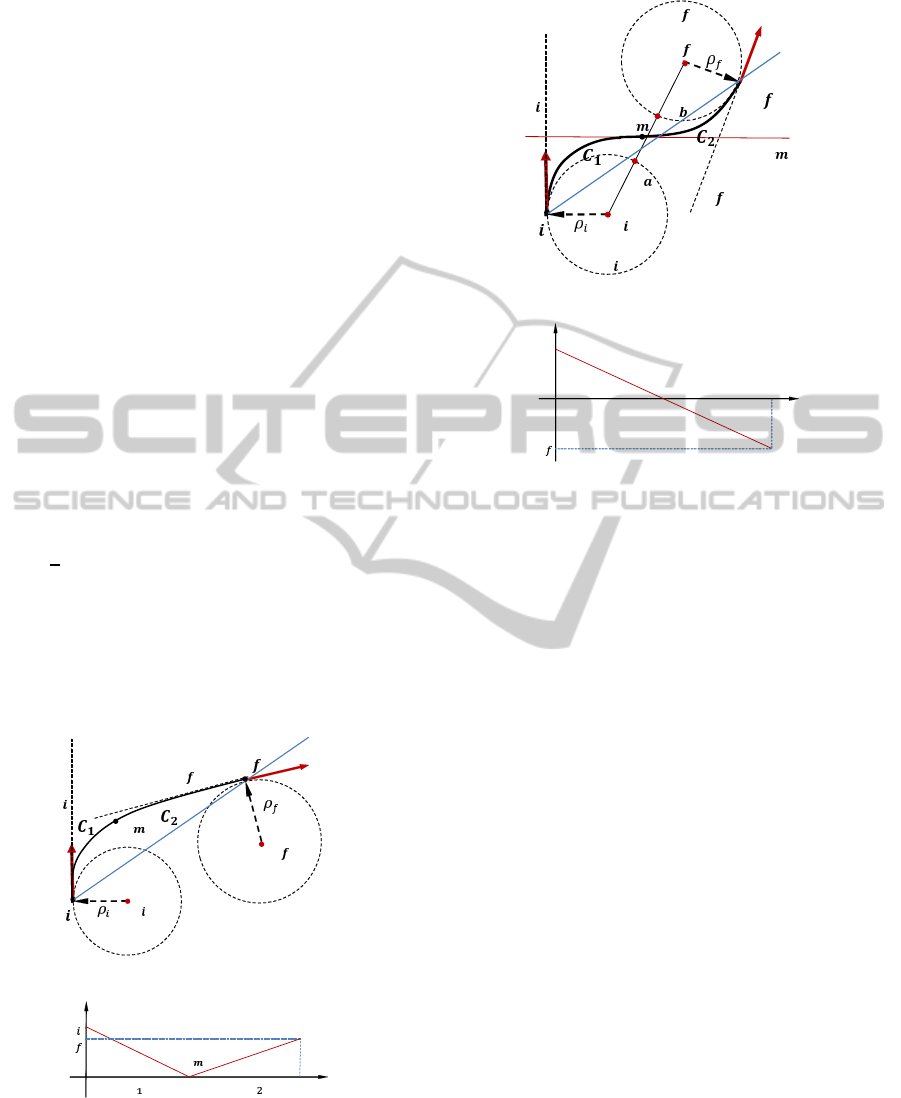
Figure 1 and Figure 2 show the path comprised by
two clothoids composition with initially same curva-
ture but with different turning direction as noted by
ࡼ
ℓ
ℓ
ℓ
ࡼ
(a) Two clothoids composition
ݏ
ߢ
ߢ
ߢ
ݏ
ଵ
ݏ
ଶ
(b) Curvature diagram
Figure 2: e-pCCP problem : C
R
1
C
L
2
.
κ
f
> 0 (cf. Figure 1) and κ
f
< 0 (cf. Figure 2) with
its corresponding curvature diagram respectively.
The initial pose P
i
and the final pose P
f
are de-
noted by vector from each end position with given
curvatures (or radius of curvature) ρ
i
and ρ
f
where
the extension lines are displayed from each pose as ℓ
i
and ℓ
f
respectively (cf. Figure 2(a)). While fulfilling
the pose configuration at both ends, clothoid segment
C
1
and C
2
(∀s ∈ [s
0
, s
l
]) are generated and located
for its final end C
1
(s
l
) to be P
i
,P
f
with same orien-
tatation of ℓ
i
and ℓ
f
. The connection point p
m
where
each orientation and curvature are same for geomet-
ric continuity is found from a parametrical adjustment
and the point can be a line depending on the config-
uration. Corresponding curvature diagram of C
R
1
C
R
2
is shown in Figure 1(b) with convention described in
Proposition 2. This diagram features the steering be-
havior while following the path, in other words, the
steering turns left from the right side position to its
center and then turns right to make another right po-
sition in steering angle. Two clothoids designate two
turning motions for steering angle and it certifies the
motion is continuous through all the travel length as
shown in curvature diagram.
Another case C
R
1
C
L
2
is shown in Figure 2. The
clothoid generation and composition procedure are
the same then the case of C
R
1
C
R
2
while satisfying the
configuration with curvature continuity. However,
different to first case, the solution of Figure 2(a) is
only available where there is sufficient space for the
SmoothTrajectoryGenerationwith4DSpaceAnalysisforDynamicObstacleAvoidance
805
line ℓ
m
to pass by between two points p
a
, p
b
that
the line c
i
c
f
and circles r
i
, r
f
meet each other. (c
i
,
c
f
are the center position of circle r
i
, r
f
.) such that
c
i
−c
f
> ρ
i
+ ρ
f
as a necessary condition.
In this case, it is required that a clothoid is supple-
mented to satisfy the two clothoids configuration.
ࡼ
ℓ
ℓ
ℓ
ࡼ
ℓ
(a) Three clothoids composition
ߢ
ߢ
ݏ
ߢ
ߢ
ݏ
ݏ
ଵ
ݏ
ଶ
(b) Curvature diagram
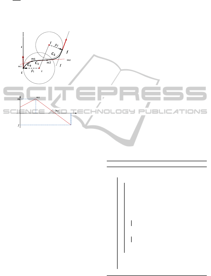
Figure 3: e-pCCP problem : C
R
0
C
R
1
C
L
2
.
Figure 3 depicts the additional case C
R
0
C
R
1
C
L
2
in-
cluding C
0
where both radius of end curvatures are
overlapped so that two clothoids can not make a meet
with each other. One of feasible method to tackle
the problem is to add a clothoid which increase from
the given initial curvature κ
i
to any higher curva-
ture κ
m
as shown in Figure 3(a). The following cur-
vature diagram of (b) explains the curvature varia-
tion of three clothoids. The resulting path of three
clothoids is useful for the dynamic obstacle planning
when the current curvature is so low (including the
case κ
i
≃ 0) that it is expected any collision with the
obstacle which is dealt with the demonstrative exam-
ples in section 4.
The detailed procedure for generating clothoids is
described in Algorithm 1 for two clothoids C
1
and C
2
that covers the cases C
R
i
C
R
f
and C
R
i
C
L
f
of (6) .
In Algorithm 1, both end curvatures κ
i
, κ
f
are
given and initial deflection δ
i
for C
1
with variations
dδ,dρ are assumed by designer before entering the
loop. In line 3, the parameter is varied according
to the property found as Properties 1 to 3 and each
clothoid is generated as given in the line 4, line 6 by
(5). The variation determinant λ(C
2
(s
0
)) for dδ is im-
portant for fast convergence with small number of it-
erations. Note that the point C
2
(s
0
) is at the other end
of C
2
since the curvature value in a clothoid is varied
from 0 to its maximum κ
max
by s
0
to s
ℓ
variation. The
rule for determining the sign of dδ is defined by an in-
equality condition which checks on the point p(x,y)
whether it locates in upper or lower side of the tan-
gential line at p
0
(x
0
,y
0
) as following.
λ(p, p
0
) = −tan(θ
i
−δ
1
)x+ y+ x
0
+ tan(θ
i
−δ
1
)y
0
(7)
where it is a straight line passing the end point
of a clothoid C
1
, i.e. C
1
(s
0
) and λ(C
2
(s
0
)) is checked
for the location on the pointC
2
(s
0
) = (x,y)|C
2
,s = s
0
.
The other determinant equation is λ
⊥
which is the per-
pendicular line of λ(C
2
(s
0
)) which is described as,
λ
⊥
(p, p
0
) = x−x
0
−tan(θ
i
−δ
1
)y
0
+ tan(θ
i
−δ
1
)y.
(8)
The composition of two clothoids by given con-
straints requires only one adjusting variable for solv-
ing the problem and there are unsolvable configura-
tions only by regulating the variable such as the end
point of C
1
locates inside of the final radius of cur-
vature circle r
f
. In such case, additional regulation
is performed to make two clothoids meet by reducing
the radius ρ
f
(or increasing the curvature) at the final
pose as described in line 13. The convergence toward
the solution is defined in line 4 where D
e
, the distance
between the composed curve C
1,2
and ℓ
m
reach the
threshold ε, e.g. 10
−3
[m].
Algorithm 1: e-pCCP generation.
Require: δ
1
,dδ, dρ
1: procedure CLOTHOID2NC(P
i
,P
f
)
2:
while D
e
≤ ε do ⊲ Dist. C
2
(s
0
) to ℓ
m
3:
δ
1
= (δ
1
+ dδ)
4: α
1
← f (κ
1
,δ
1
) ⊲ C
1
generation
5:
δ
2
= θ
i
−θ
f
−δ
1
⊲ G
2
continuity
6: α
2
← f
′
(κ
2
,δ
2
) ⊲ C
2
generation
7:
D
e
← ℓ
m
,C
2
(s
0
)
8: dδ = sign(λ)|dδ|
9:
if λ(C
2
(s
0
))
¯
λ < 0 then
10: dδ = dδ/2
11:
end if
12: if λ
⊥
(C
2
(s
0
))
¯
λ
⊥
< 0 then
13:
ρ
f
= ρ
f
−dρ ⊲ ρ
f
reduction
14: end if
15:
¯
λ = λ,
¯
λ
⊥
= λ
⊥
16: end while
17:
e
C ←C
1
⊕C
2
⊲ Composition: ⊕
18:
return
¯
α
sol
,
e
C(
¯
α
sol
) ⊲ Obtained Solution
19: end procedure
ICINCO2014-11thInternationalConferenceonInformaticsinControl,AutomationandRobotics
806

3 VELOCITY PLANNING IN 4D
SPACE
3.1 4D Space Analysis for Obstacle
Avoidance
In this subsection, a framework of 4D space is in-
troduced to analyze collision detection in space and
time domain and to plan the obstacle avoidance ma-
neuver for a vehicle. Cartesian coordinated 3D con-
figuration space (C-space) with additional time axis
are constructed to analyze future status for dynamic
objects. A representative description is shown in Fig-
ure 4 where two vehicle move in each direction and
expected to make collision on intersection at a colli-
sion time t
c
by meeting the two future trajectory lines
L
a
and L
b
. It is shown that an obstacle vehicle moving
in velocity v
a
and a vehicle of v
b
collide at the state
S
c
in 4D space. In 4D space, it is easy to check on any
possible collision among dynamic objects by measur-
ing minimum distance between each future trajectory
line whether the resultant value is less than a collision
threshold distance where the threshold is bounded by
object modeling scheme.
With 4D analysis and circular representation for
the vehicle, feasible avoidance pose can be deter-
mined to avoid any collision by replanning the trajec-
tory. One of possible avoidance plan is to modify the
velocity profile by encompassing the collision bound-
ary with minimal changes of original velocity profile.
The other possible avoidance consists to set up the
arrival pose of the future generating path to be safe
from any collision. For the dynamic obstacle avoid-
ance, here, two avoidance poses (front and rear) are
considered as follows.
Figure 5 presents the collision plane of the ob-
stacle where the horizontal axis corresponds to the
configuration space C and vertical axis presents fu-
ture time. Consistent with the problem definition,
the obstacle is assumed to move from left side of
Figure 4: 4D configuration analysis for collision avoidance.
Obstacle
ࡼ
ࢉ
ࡼ
ࢌࢇ
ࡼ
࢘ࢇ
࢚
ࢉ
܀
۴
ܚ
ԧ
࢚
ࡿ
ࢉ
ࡸ
ࢌ
ࡸ
࢘
۴
ത
ܚ
܀
ഥ
Figure 5: Avoidance pose planning in collision plane.
the line ℓ
i
(cf. Figures 1,2 and 3) to right side with
constant velocity (same speed and orientation) at t
1
.
This methodology remains effective when the obsta-
cle changes its orientation or speed such that replan-
ning is started as the change is detected. At the posi-
tion of P
c
in t
c
, a collision is expected at the state S
c
.
In the plane, there are two avoidance modes accord-
ing to the location of the obstacle boundaries. Upper
region of the boundary, noted as L
f
corresponds to
front avoidance region and lower part of the bound-
ary L
r
corresponds to rear avoidance. The avoidance
pose (or final pose) P
f
is determined to be the point on
the tangential line which is perpendicular to obstacle
velocity direction. According to the avoidance pose,
the path by the vehicle is C
R
1
C
R
2
for L
r
andC
R
1
C
L
2
for L
f
avoidance.The vehicle is represented by two circles in
this work to simply check the collision distance with
obstacles. When the obstacle comes close to collide
with the vehicle from the right side to left of ℓ
i
(cf.
Figures 1,2 and 3), the avoidance modes are changed
each other with the same scheme. Under two avoid-
ance shemes of velocity replanning and path replan-
ning, there are four avoidance statuses
¯
F
r
,
¯
R
f
, F
r
and
R
f
where every subscript signifies colliding obstacles
(circle) with one of the two circles (which surround
the vehicle).
Note that
¯
F
r
,
¯
R
f
in velocity change avoidance lo-
cate at the vertical line of P
c
where both circles pass
by the expected collision position P
c
but with arrival
time differences. For the path replanning, it requires
another stragegy to constrain the arrival time at rear
avoidance arrival pose P
ra
or front avoidance arrival
pose P
fa
. In what follows, the strategy to locate the
collision time t
c
to be out of the obstacle boundary is
to find the time at avoidance pose F
r
or R
f
which are
in the same level of t
c
as well as being closest to the
obstacle boundary. In the avoidance maneuver, the
initial velocity at t
i
could be maintained with a little
changes according to the changes in the travel length
of the new replanned path.
3.2 Dynamic Obstacle Avoidance
With the obtained solution for path planning, using
SmoothTrajectoryGenerationwith4DSpaceAnalysisforDynamicObstacleAvoidance
807
clothoids given in section 2.3, it is proposed in this
section to apply it for dynamic obstacle avoidance
problem. In the dynamic obstacle problem, the ob-
stacle is represented with a circle (Chakravarthy and
Ghose, 2011) having constant velocity.
With the configuration described in section 2.3, e-
pCCP to avoid obstacles is generated.
P
i
P
f
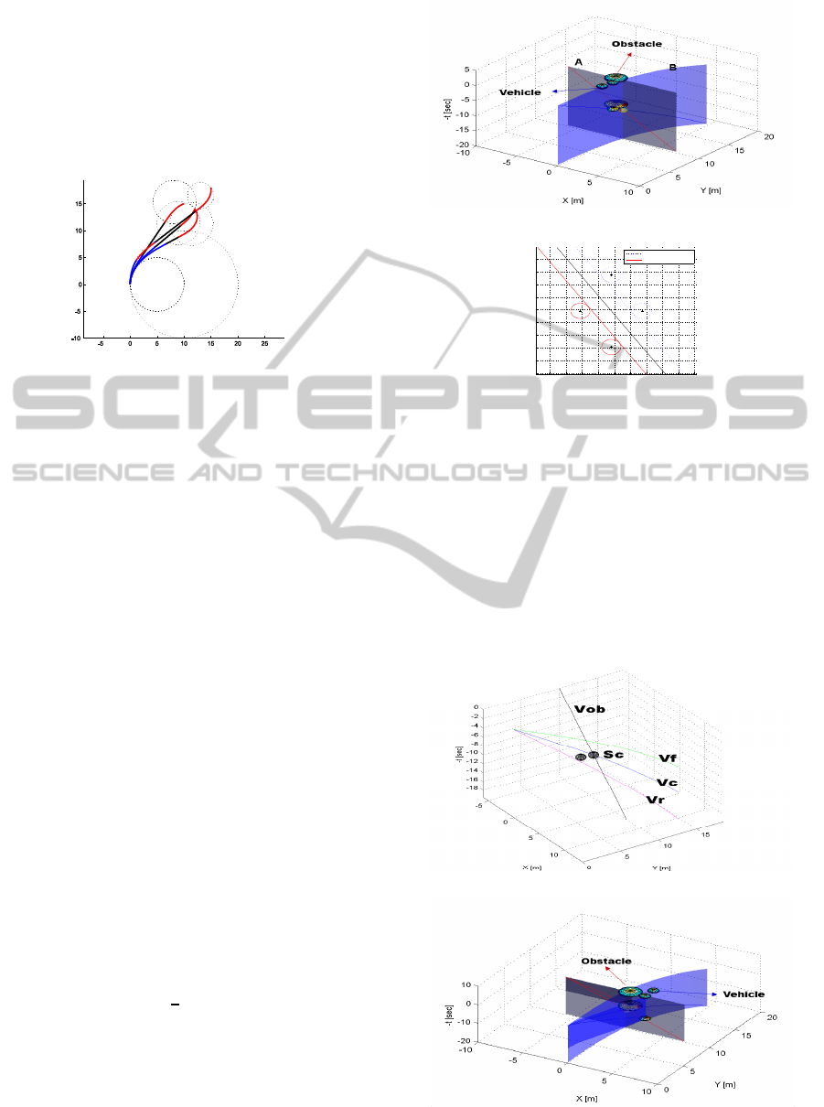
Figure 6: e-pCCP for obstacle avoidance.
In Figure 6, four different configurations are ap-
plied for e-pCCP generation. Each generated path sur-
round the obstacle circle to avoid the obstacle by path
following. The initial configuration and final configu-
ration are denoted by P
i
and P
f
while the correspond-
ing radius of curvatures are presented respectively.
The generated paths are composed by two clothoid
with additional straight line to have curvature conti-
nuity while avoiding the obstacle boundary as close
as possible. This avoidance path has additional ad-
vantages as follows. At first, the path could be short
accoring to the static or dynamic obstacle. Secondly,
the rate of steering turn (or sharpness) is minimal
compared to farther pose avoidance from the obsta-
cle. Lastly, such path could be still efficient when the
obstacle changes its moving direction while avoidng
since the path could be also regenerated with current
steering angle as initial curvature and new final con-
figuration by expected obstacle motion. Obtained e-
pCCP is applied in 4D configuration space in order
that the path combines the velocity smoothness for
dynamic obstacle to fulfill the continuous trajectory
of vehicles.
Figure 7 presents a demonstrative 4D space sim-
ulation for dynamic obstacle avoidance. In (a), the
obstacle trajectory of A plane and the vehicle trajec-
tory of B plane are plotted in the space by given infor-
mation for the obstacle P
A
i
(−6,10,0, 0) with 0.6 m/s
and the vehicle P
B
i
(0,0,
π
2
,0.08). In this configura-
tion, a collision is predicted at 10 sec in future and (b)
depicts the obstacle avoidance poses determination as
described in Figure 5.
Figure 8 shows the replanned trajectory for the
simulation given in Figure 7 where (a) is the velocity
replanning and (b) is the replanned path by e-pCCP.
In (a), collision state S
c
is shown along the trajec-
(a) Collision case
3 4 5 6 7 8 9 10 11 12
−15
−14
−13
−12
−11
−10
−9
−8
−7
−6
Travel length [m]
Elapsed time [−sec]
Front avd.(Rear circle)
Rear avd.(Front Circle)
(b) Avoidance planning
Figure 7: 4D analysis for dynamic obstacle avoidance.
tory line v
c
with obstacle trajectory v
ob
. For the ve-
hicle, the front avoidance with current velocity v
f
and
rear avoidance with current velocity v
r
are planned
while both avoidance trajectories keep the safe dis-
tance to avoid any collosion with the obstacle trajec-
tory. Figure 8(b) demonstrates that the generated tra-
jectory guarantees a smooth collision avoidance with
the dynamic obstacle.
(a) Velocity replanning
(b) Safe trajectory
Figure 8: e-pCCP for obstacle avoidance.
ICINCO2014-11thInternationalConferenceonInformaticsinControl,AutomationandRobotics
808

4 CONCLUSIONS
This paper presents a smooth trajectory generation for
dynamic obstacle with 4D space analysis and e-pCCP.
Extending pCCP to the nonzero curvatures problem
permits the generated path to be reactive for dynamic
obstacle. By collision checking in 4D space analysis
with two circles vehicle representation for the vehicle,
the avoidance poses are determined to avoid any risk
of collision on the future. The resultant trajectory has
steering smoothness on the path as well as smooth ve-
locity changes along the path. Demonstrative exam-
ples on a dynamic obstacle shows the effectiveness
of the proposed methods and expected to be imple-
mented for more complicated dynamic environments
such as multiple obstacles or cluttered areas with real
time performance.
REFERENCES
Adouane, L. (2013). Toward smooth and stable reactive mo-
bile robot navigation using on-line control set-points.
In IEEE/RSJ, IROS’13, 5th Workshop on Planning,
Perception and Navigation for Intelligent Vehicles,
Tokyo-Japan.
Berg, J. V., Lin, M., and Manocha, D. (2008). Recipro-
cal velocity obstacles for real-time multi-agent navi-
gation. IEEE Int. Conf. on Robotics and Automation,
pages 1928–1935.
Chakravarthy, A. and Ghose, D. (1998). Obstacle avoidance
in a dynamic environment: A collision cone approach.
IEEE trans. on Systems, Man and Cybernetics-Part A:
Systems and Humans, 28(5):562–574.
Chakravarthy, A. and Ghose, D. (2011). Collision cones
for quadric surfaces. IEEE Trans. on Robotics,
27(6):1159–1166.
Dubins, L. E. (1957). On curves of minimal length with a
constraint on average curvature, and with prescribed
initial and terminal positions and tangents. American
Journal of Mathematics, 79:497–516.
Fiorini, P. and Shiller, Z. (1998). Motion planning in dy-
namic environments using velocity obstacles. Int. J.
of Robotics Research, 17(7):760–772.
Fraichard, T. and Scheuer, A. (2004). From Reeds and
Shepp’s to continuous curvature paths. IEEE Trans.
on Robotics, 20:1025–1035.
Fulgenzi, C., Spalanzani, A., and Laugier, C. (2007). Dy-
namic obstacle avoidance in uncertain environment
combining pvos and occupancy grid. IEEE Int. Conf.
on Robotics and Automation, pages 1610–1616.
Giesbrecht, J. (2004). Global path planning for unmanned
ground vehicles.
Gim, S., Adouane, L., Lee, S., and Derutin, J.-P. (2014).
Parametric continuous curvature trajectory for smooth
steering of the car-like vehicle. Int. Conf. on Intelli-
gent Autonomous Systems.
Kelly, A. and Nagy, B. (2003). Reactive nonholonomic
trajectory generation via parametric optimal control.
The International Journal of Robotics Research, 22(7
- 8):583 – 601.
Khatib, O. (1986). Real-time obstacle avoidance for ma-
nipulators and mobile robots. The int. J. of Robotics
Research, 5(1):90–98.
Labakhua, L., Nunes, U., Rodrigues, R., and Leite, F. S.
Smooth trajectory planning for fully automated pas-
sengers vehicles: Spline and Clothoid based methods
and its simulation.
Lamiraux, F. and Laumond, J. P. (2001). Smooth mo-
tion planning for car-like vehicles. IEEE Trans. on
Robotics and Automation, 17(4):498–501.
Likhachev, M. and Ferguson, D. (2009). Planning long dy-
namically feasible maneuvers for autonomous vehi-
cles. Int. Journal of Robotics Research, 28(8):933–
945.
Montes, N., Mora, M. C., and Tornero, J. (2007). Tra-
jectory generation based on rational Bezier curves as
clothoids. IEEE Intel. Vehicles Symposium, pages
505–510.
Reeds, J. A. and Shepp, L. A. (1990). Optimal paths for
a car that goes both forwards and backwards. Pacific
Journal of Mathematics, 145(2):367–393.
Solea, R. and Nunes, U. (2006). Trajectory planning with
velocity planner for fully-automated passenger vehi-
cle. Intel. Transportation Systems Conf., pages 474–
480.
Thompson, S. and Kagami, S. (2005). Continuous curva-
ture trajectory generation with obstacle avoidance for
car like robot. Int. Conf. on Computational Intelli-
gence for Modeling, Control and Automation, pages
863–870.
Villagra, J., Milantes, V., Perez, J., and Godoy, J. (2012).
Smooth path and speed planning for an automated
public transport vehicle. Robotics and Autonomous
Systems, 60:252–265.
Wilde, D. K. (2009). Computing clothoid segments for
trajectory generation. IEEE/RSJ Int. Conf. on Intel.
Robots and Systems, pages 2440–2445.
Wilkie, D., van den Berg, J., and Manocha, D. (2009). Gen-
eralized velocity obstacles. IEEE Int. Conf. on Intelli-
gent Robots and Systems, pages 5573–5578.
Wu, P. P. Y., Campbell, D., and Merz, T. (2011). Multi-
objective four-dimenstional vehicle motion planning
in large dynamic environments. IEEE Trans. on
Systems, Man, and Cybernetics-Part B:Cyberntetics,
41(3):621–634.
SmoothTrajectoryGenerationwith4DSpaceAnalysisforDynamicObstacleAvoidance
809
