
CFD Prediction of the Effect of Appendages and Leeway on the Force
Trend of an Olympic Class Laser Dinghy Hull
Rickard Lindstrand
1
, Jeremy Peter
1
and Christian Finnsgård
2,3
1
Department of Shipping and Marine Technology, Chalmers University of Technology, Gothenburg, Sweden
2
SSPA Sweden AB, Research, Gothenburg, Sweden
3
Centre for Sports Technology, Department of Applied Physics, Chalmers University of Technology, Gothenburg, Sweden
Keywords: CFD, Sailing, Verification & Validation, Tow Tank Testing.
Abstract: The purpose of this paper is to investigate whether the minima in hydrodynamic resistance can be predicted
to occur at the same angles of heel and trim in the case of bare hull towing tank tests, bare hull simulations
and appendage and leeway simulations. If so, the appendages and the leeway can be rejected from future
investigations, which would prove a beneficial advancement, as they impose further complexity to
simulations. The results of verification and validation (V&V) included in this paper demonstrate that the
numerical method predicted too low resistance. Though the study identifies and systematically investigates
possible sources of error, the major source of error was not found. These various possible sources of errors
were identified for further research, and as future references for similar cases. Moreover, the simulation
results for the variations of heel and trim also require further study. Before a full set of results is available,
one cannot make conclusions regarding the angles of heel and trim that lead to minimal resistance. This
paper discusses the results and potential avenues of future research, and is a result of an initiative at
Chalmers University of Technology focusing on sports and technology.
1 INTRODUCTION
As a result of the hull’s complex three-dimensional
shape, the flow around the dinghy will differ for
different attitudes to the direction of motion. This
implies the possibility of locating a minimum of
hydrodynamic resistance by sailing at a specific
angle of trim and heel. Finding the attitude of
minimum resistance can potentially increase
performance.
Hydrodynamic resistance is not the only effect
that must be considered when altering the angle of
heel and trim. The projected area for the centerboard
and rudder is decreased when the dinghy is heeled,
and this is the case for the sail as well. Moreover,
stability could be decreased when trimming on the
bow. These effects will not, however, be taken into
account in this paper.
Since the weight of the sailor represents more
than half of the displacement, the angles of heel and
trim are changed by positioning the dinghy’s sailor
in a certain manner.
At the professional level sailors perform
similarly, and thus possibilities like the sailor’s
position must be exploited in order to gain
advantage on the race course. There is little evidence
in the literature that an investigation along these
lines has been conducted before.
The hull used for this study is the Laser dinghy
(see www.laserinternational.org for a description), a
four-meter-long dinghy for one sailor. The Laser
class has been an Olympic discipline since the 1996
Summer Olympics in Atlanta, and is a strict one-
design class, which means that design alterations or
additions of any kind are prohibited. Therefore, the
manner in which the dinghy is sailed becomes ever
more important, and any improvements in sailing
practice will consequently improve performance in
competitive situations at the international level.
The study resulting with the current paper is a
part of an initiative at Chalmers University of
Technology. The Olympic motto, “Citius, Altius,
Fortius” (Latin for “Faster, Higher, Stronger”),
governs everyday life for many engineers, and for
the last few years Chalmers has supported a project
that focuses on the possibilities and challenges for
research combined with engineering knowledge on
the area of sports. The initiative has generated
190
Lindstrand R., Peter J. and Finnsgård C..
CFD Prediction of the Effect of Appendages and Leeway on the Force Trend of an Olympic Class Laser Dinghy Hull.
DOI: 10.5220/0005191101900202
In Proceedings of the 2nd International Congress on Sports Sciences Research and Technology Support (icSPORTS-2014), pages 190-202
ISBN: 978-989-758-057-4
Copyright
c
2014 SCITEPRESS (Science and Technology Publications, Lda.)

external funding and has gained great acclaim within
Chalmers, among staff and students, in the Swedish
sports movement, in large companies, as well as
within SME’s. The project focuses on five sports:
swimming, equestrian, floorball, athletics, and
sailing.
The paper is composed as follows: Chapter 1
provides the background to the problem and a very
brief introduction to the basics of the mechanisms of
sailing, the methodology and tow tank test setup.
Chapter 2 governs the computational method, while
Chapter 3 adresses the numerical method. Chapter 4
and 5 recites the verification and Chapter 6 the
validation. Chapter 7 finalises the paer with the
concluding remarks.
1.1 Background
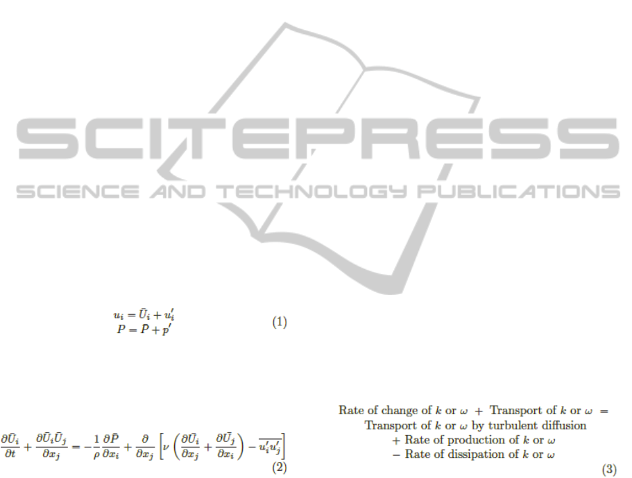
The governing equations for the dynamics of a fluid
are the Navier-Stokes equation (NS) and the
continuity equation. However, it is not possible to
fully resolve the flow around a ship, yacht or dinghy
with these equations (Larsson and Raven, 2010,
section: 9.7.1). This is due to the large separation of
scales in the domain and the computational effort
required to handle such a separation. While the
Laser dinghy is four meters long, the smallest scales
in the flow, the Kolmogorov scales, are a mere
fraction of a millimetre (Larsson and Raven, 2010).
As a result, the resolution of the discretized domain
must be incredibly fine in order to fully resolve the
flow (Feymark, 2013). The resolving of one of the
smallest turbulent scales requires approximately four
cells in each spatial direction.
For ship applications, the level of resolution must
therefore be limited to that which results in an
affordable number of cells. An increase in the cell
size leads to a loss of information regarding the
smaller turbulent structures. To compensate for this
loss of information, turbulence models and near-wall
function are introduced to the simulation.
Meanwhile, the temporal resolution is neglected all
together, as the flow’s average quantities are of
greater interest than its instant ones (Larsson and
Raven, 2010). For example, it may be more valuable
to know the average hydrodynamic resistance, rather
than the value at each hundredth of a second.
One criterion for neglecting the temporal
discretization is that the flow is considered steady, or
independent of time. The equations must therefore
be adjusted in order to handle averaged quantities.
This operation is called Reynolds time averaging,
and the new equation is termed the Reynolds time-
averaged Navier-Stokes equation (RANS). As the
flow case of the dinghy in flat water is in fact one of
steady flow, this paper will employ RANS
equations.
1.2 Mechanisms of Sailing
The sail can be understood as a thin wing profile.
The wing generates lift and drag, which are defined
as the force components that are perpendicular and
parallel, respectively, to the apparent wind. The
apparent wind is the wind experienced by the sail,
i.e., with the boat velocity included (see Figure 1).
The point at which the pressure field of the sail can
be substituted by one force vector is called the center
of effort. As the center of effort is dependent on the
pressure distribution, it is not easy to identify,
though its location can be estimated at the sail’s
surface center.
Figure 1: Wind speeds and directions. The leeway is the
difference between the heading and the true boat velocity.
The lift of the sail is the only component acting
in the yacht’s positive direction of motion, and is
therefore the only component contributing to
propulsion. Furthermore, only one component of the
lift is in turn completely aligned with the direction of
the yacht. In order for the yacht to move in the right
direction, this driving force component must balance
the hydrodynamic resistance of the hull, the
component of the drag generated by the sail aligned
with the opposite direction of the yacht, and the drag
generated from the rigging, deck equipment, etc.
The term leeway refers to the slight drift of a
moving sailing craft toward the leeward side, and is
the result of the misalignment of the resultant force
of the sail and the direction of motion. This drift is
angled in the leeward direction, hence the name
leeway. As the center of effort of the sail is not at the
same height as the center of pressure for the hull and
keel, a heeling moment will also be generated,
resulting in the heel angle.
CFDPredictionoftheEffectofAppendagesandLeewayontheForceTrendofanOlympicClassLaserDinghyHull
191

1.3 Methodology
Prior to the investigation of heel and trim variations,
a V&V study will be performed. This verification
and validation study will be conducted in order to
identify the amount of error to be expected from the
simulations, and consequently, their relative
trustworthiness. Section 4 will further explain the
verification procedure.
1.4 Towing Tank Test Setup
Preparation of the dinghy for tow tank testing
necessitated modifications. An aluminium frame
was fitted to the deck around the cockpit. This frame
provided a point at which to attach the towing device
and also served to accommodate the weights used to
position the dinghy in the desired attitude. The
appendages were also removed in order to facilitate
what will be called a bare hull case. The final
modification consisted of the addition of points at
which to attach string connected to the measuring
devices used to accurately measure heel and trim
during speed tests. Figure 2 display the test frame on
the deck.
Figure 2: Display of the towing tank test Laser. Photos by
SSPA.
The towing device is attached to the top of the
vertical aluminium profile. As the towing force is
not applied through the center point of the
hydrodynamic resistance, a trimming moment is
hereby introduced. This moment will not be similar
to an actual sailing case, as the towing point does not
coincide with the sail’s center of effort.
The arm of the towing devise was set up so as to
be horizontal for the static cases. This meant that at
higher speeds when the dinghy meets with a
considerable draft change, the arm would no longer
be horizontal, and the towing force would pull the
dinghy slightly downward. This would create an
increase in displacement, which would in turn affect
resistance. Thus, the simulations to be performed
could not be set to free sinkage and trim.
Due to limited testing time, the heel tests were
only performed as heel to starboard tests.
The brackets that help hold the frame in place are
located on the railing of the dinghy, as illustrated in
Figure 2b. As the heel angle increased, the starboard
side brackets began interfering with the spray from
the bow wave. They were therefore removed from
that side and from the test rerun, without
interference from the frame.
During the test runs, a bailing pump was added
on the flooring of the cockpit to guard against excess
water. This excess water was a product of the not
completely watertight self-bailer device, which was
given to leak by the reversal of the test setup back to
the starting position in the towing tank after each
run.
2 COMPUTATIONAL METHOD
2.1 Governing Equations
The equations that govern fluid flow are derived
from basic physical principles and described by the
mathematical statements of the conservation laws of
physics: the conservation of mass and momentum.
The Navier-Stokes equations are derived from the
conservation laws and from several underlying
assumptions, and are used to predict the resistance
forces that result from water pressure and viscous
effects.
Basic assumptions. The Navier-Stokes
equations are based on the assumptions that the fluid
is a continuum, that is, a continuous substance, as
opposed to an aggregate of discrete particles.
In the case of water, the flow is commonly
considered incompressible, rendering constant the
density ρ and the viscosity µ.
The Navier-stokes equation is then time averaged
in order to arrive at the RANS equation
Coordinate system. The simulations are not set
up to account for changes in sinkage or trim, as a
result of the unnatural trimming moment and the
vertical force component created by the towing
device. The simulation is also assumed to be steady,
that is, it is assumed the dinghy will not move
relative to waves or in time. In the global Cartesian
coordinate system employed here, the origin is at the
icSPORTS2014-InternationalCongressonSportSciencesResearchandTechnologySupport
192
bow on the centerline at the undisturbed water level,
x is directed sternward, y is directed starboard and z
is directed vertically upward.
2.2 Turbulence
2.2.1 Turbulent Flow
Typically, the fluid flow around the hull of a moving
ship is turbulent. Turbulent flows are irregular,
random and three-dimensional. In such flows,
velocity and pressure change continuously, creating
within the flow a spectrum of turbulent structures.
Despite the irregular nature of a turbulent flow, it is
possible to resolve its behaviour with the Navier-
Stokes equations (Davidsson, 2003). However,
doing so requires that the spatial and temporal
discretizations are capable of capturing all scales in
the flow. This is not possible for ship applications,
as the smallest scales are minuscule in relation to the
length of the hull, and this in turn leads to
unreasonable computational effort.
To resolve the turbulent flow at issue in the cases
here, this study utilizes the Reynolds-averaged
Navier-Stokes equation (RANS). This requires that
the regular Navier-Stokes equations are averaged
over time, a task accomplished by decomposing the
instantaneous variables into a mean value and a
fluctuating value ϕ′ :
Insertion of the decomposed terms from (1) into the
Navier-Stokes equations gives rise to the Reynolds-
averaged Navier-Stokes (RANS) equations. The
expression of the incompressible Newtonian fluid in
the Einstein notation is:
This allows for more attention to the mean values,
and less to the time histories; indeed, when solving
the Navier-Stokes equations, a very fine resolution
in time would be necessary in order to resolve the
unsteady turbulent flow.
2.2.2 Modelling Turbulence
In the equation (2) the term ′
′
appears from the
fluctuating values. Known as the Reynolds Stress
tensor, this term is an unknown. In order to close the
equation system and solve for all the unknowns, the
Reynolds stress tensor must be modelled. This is
commonly termed the closure problem.
There are various ways to model the Reynolds stress
tensor, including the use of algebraic models, one-
equation models, two-equation models, algebraic
stress models and Reynolds Stress models. Each of
these turbulence models varies in terms of
computational requirements, accuracy in turbulence
modelling and complexity.
Two turbulence models were implemented in the
software i: the two-equation Menter’s Shear Stress
Transport model (SST k-ω) and the explicit
algebraic stress model (EASM). A description of
these models is available below.
Menter’s SST k-ω model. Menter proposed the
SST k-ω model in 1992 in order to improve the
performance of the near-wall turbulence modelling
of the commonly used two-equation k-ε-model
(Menter, 1994). The SST k-ω model uses the
turbulent kinetic energy k, the turbulence frequency
ω = ε/ k (dimension: s
-1
) and the Boussinesq
assumption to compute the Reynolds stresses. The
Boussinesq assumption is the presumed relation
linking the Reynolds stress tensor to the velocity
gradients and the turbulent viscosity. When a
turbulence model uses the Boussinesq assumption, it
then qualifies as a “linear eddy viscosity model”.
This two-equation turbulence model uses one
modelled transport equation for each of the two
variables, k and ω. The ω-equation is derived from
the ε-equation in the k-ε-model by simply
substituting the relation ε=kω. Though these
equations are not displayed here in detail, it is
nevertheless important to understand the manner in
which these transport equations are constructed. For
both equations, the structure is as follows (Versteeg
and Malalasekera, 2007):
The SST k-ω model combines the benefits of the
Wilcox’s k-ω model at the near-wall and the
performance at the freestream and shear layers of the
k-ε model. This is why Menter’s SST k-ω model is
suitable for a wide range of CFD applications
(Rumsey, 2013). Additionally, assessments of this
turbulence model have suggested that it offers
superior performance in the case of an adverse
pressure gradient boundary layer (Versteeg and
Malalasekera, 2007). An adverse pressure gradient
leads to lower kinetic energy of the fluid, and hence
to a reduction of its velocity. If the pressure increase
is large enough, the fluid direction can be reversed;
this is what occurs in flow separation, a phenomenon
CFDPredictionoftheEffectofAppendagesandLeewayontheForceTrendofanOlympicClassLaserDinghyHull
193

that typically occurs at the transom of a boat like the
Laser. Therefore, this turbulence model seems to be
well suited for the current CFD application..
EAS Model. The Explicit Algebraic Stress
Model (EASM) proposed in Wallin and Johansson
(2000) provides an alternative to linear eddy
viscosity models (such as the SST k-ω) based on the
Boussinesq hypothesis. Often, linear eddy viscosity
models fail to offer satisfactory predictions for
complex three-dimensional flows, due to the
involvement of the Boussinesq assumption. This
leads to nonlinear stress-strain relations in
turbulence modelling that contradict the Boussinesq
assumption. (Gatski and Speziale, 1993).
Nevertheless, owing to their high level of stability,
these linear eddy viscosity models are commonly
used in the industry (Versteeg and Malalasekera,
2007).
The original algebraic stress model (ASM)
model is not often used as a result of robustness
issues and frequent instances of singular behaviour
(Deng, Queutey, and Visonneau, 2005), both of
which the EAS Model addresses by suggesting
treatment of the non-linear term by the production-
to-dissipation rate ratio, and the number of tensor
bases used to represent the explicit solution of those
equations. Gatski and Speziale (Gatski and Speziale,
1993) have identified an exact solution for three-
dimensional flow involving a ten-term tensor, but
require too much computational power. Alternatives
discerns that five terms yields acceptable
approximation of the solution to the algebraic stress
equation (Deng, Queutey, and Visonneau, 2005).
2.3 The Volume of Fluid Method, VOF
The VOF method is a multiphase flow method that
computes the interaction of several fluids or phases
of a fluid present in the same domain, and obtains
the interface between these fluids (Marek,
Aniszewski and Boguslawski, 2008). For the
purposes of yachting applications, implementation
of this method allows for the accurate inclusion of
the computation of the free water surface around the
hull of the yacht.
The VOF method calls for the solving of, the
same Navier-Stokes equation as do single-phase
flows. The difference lies in a phase indicating
function γ (Hirt and Nichols, 1979). This phase,
called the colour function or volume fraction,
displays the measure of the mixture of phases in
each cell. For instance, if γ = 1, the cell is
completely occupied by phase one, and if γ = 0.3,
30% of phase one and 70% of phase two are present
in the cell. In terms of yachting applications, the two
present fluids are water and air. As air is included in
this method, the spatial discretization must extend
above the waterline as well. This does, of course,
increase the computational effort of the simulation,
but it offers a significantly more accurate physical
representation of the waves, as will be explained
below.
The physical fluid properties used in the Navier-
Stokes equation for a multiphase flow is a blend of
the properties of the present fluids. In the case of
yachting, in which the present fluids are air and
water, the computational properties are blended in
the following manner:
To track the motion of the interface, a separate
transport equation for the colour function is used:
This method does, however, give rise to a
numerical problem regarding the smearing of
boundaries between the phases over several cells.
This smearing denotes that the water surface is
constituted by a gradual change in density between
water and air. As the water surface is a discontinuity,
a jump in density, this smearing represents an
unwanted phenomenon. It is a result of the
convective averaging being conducted across the
water surface. The remedy for this smearing is to
implement, in the code, a way to detect the presence
of a boundary (Hirt and Nichols, 1998) and treat the
bounded areas separately. In the Shipflow software,
the smearing problem is addressed by
implementation of a compressive discretization
scheme, as suggested by Orych, Larsson and
Regnstrom (2010).
To render visible the surface of the water, the
distribution of the colour function is evaluated.
Where 0<γ<1 there is a mixture between the fluids
and the free water surface is found. As mentioned,
however, the boundary between the phases may be
smeared, and therefore a specific value of γ is
selected to display the surface.
The VOF method belongs to the class of surface
capturing methods. In such methods, the interface
between two fluids is computed somewhere inside
the domain. The main difference from single-phase
surface tracking methods is that, in this case, the
dynamics of the air are also computed. In single-
phase methods, the water surface geometry forms
the top boundary of the domain, and thus these
icSPORTS2014-InternationalCongressonSportSciencesResearchandTechnologySupport
194

methods do not take the air into account. The
geometry of the top of the domain is then in every
time step or iteration updated according to the
kinematic and dynamic free surface conditions, and
a new grid with new top geometry is generated for
the next iteration (Lasson and Raven, 2010). In the
VOF method, the free surface conditions are
automatically satisfied. Furthermore, surface
capturing methods have the advantage of being able
to capture overturning waves, drops and complex
surface features, if the resolution of the grid is fine
enough.
For the purposes of this paper, the advantages of
the VOF method in the form of physical
representation outweigh the disadvantages of
computational cost and numerical instability, and the
VOF method will therefore be used for all resistance
computations.
3 NUMERICAL METHOD
3.1 Description of the Computational
Domain
A structured H-O-grid defines the domain around
the hull. This grid layout is desirable because it will
generate cells that are roughly aligned with the
direction of the flow and fitted to the geometry.
Three different structured grids—the H-O-grid,
H-H-grid and O-O-grid—are used to cover each part
of the domain. The grid type refers to the shape of
the overall domain. The first two grid layouts are
displayed in Figures 5a and 5b, respectively. The
dome-shaped O-O-grid, used around the
appendages, is illustrated by Figure 4b.
The near-wall cells must be quite thin to allow
for representation of the velocity profile in the
boundary layer, as the gradient of the velocity
profile defines the amount of viscous resistance. No
wall function was used. The near-wall cells
distribution can be observed in Figure 3.
Figure 3: Display of cell density near the walled boundary
of the hull.
The H-O-grid layout is used, as displayed in Figure
5a, only in the verification and validation phase, as
the hull is then oriented straight against the flow,
which means that the case is symmetric. In these
cases, the simulations are also symmetric along the
centerline.
The H-H-grid, also called box, is used as the
main structure for the simulations of the heel and
trim variations. Figure 5b demonstrates this grid
layout. The geometrical representation of the
dinghy’s hull and appendages was then added to the
domain in the form of overlapping component grids.
When these component grids were added, they were
also given the selected angles of heel and trim
corresponding to the ones obtained at speed during
the towing tank tests.
Figure 4: Display of the subgrids used for the investigation
cases with appendages and leeway.
Figure 5: Overview of grid types.
3.2 Boundary Conditions
The boundary conditions for the domain are
displayed in the following figure. The slip boundary
condition is in practice the same as symmetric,
which is why the symmetry boundary is also marked
slip. The space above and behind the dinghy is also
discretized in two separate grid blocks which are
removed from the figure for better visibility.
Figure 6: Boundary conditions for the symmetric domain.
The same boundary definition is valid for the boxed grid.
CFDPredictionoftheEffectofAppendagesandLeewayontheForceTrendofanOlympicClassLaserDinghyHull
195

4 VERIFICATION METHOD
As the governing equations are implemented in a
computer code, the fields of the flow properties must
be discretized into smaller fluid particles to which
the equations are then applied. The differential
equations must be linearized and schemes must be
applied in order to estimate the derivatives. The size
of the cells in the domain impacts the flow’s
representation. In general, the smaller the cells, or
the larger the amount of cells in the domain, the
better the representation of the flow field (Versteeg
and Malalasekera, 2007). The number of cells will
influence to a great degree just how computationally
demanding the simulation will be.
The flow properties are stored in the center of
each cell. The cells interact, however, by way of
their adjoining boundaries, which means that the
quantities must be interpolated to the boundary from
the centers. This is done according to an
interpolation scheme implemented in the code. To
determine how well the interpolation scheme is
performing in terms of accuracy, a Taylor expansion
of a convective term (a derivative) is conducted
(Versteeg and Malalasekera, 2007). When the low
order terms are cancelled, the one left with the
lowest degree of dependency on the cell size defines
the scheme’s order of accuracy. The higher order
terms in the Taylor series are neglected and the sum
is truncated so as to only contain the one defining
term.
However, the theoretical order of accuracy, or
the decrease in error, might not be observed when
refining the grid. This may be attributable to the fact
that the refinement of the grid is not completely
uniform, to the fact that the wall distance necessary
for a turbulence model to be activated is not scaled
correctly, or to the fact that the aspect ratio of the
cells may change. One further explanation for the
inability to obtain the theoretical order of accuracy is
that the truncated higher order terms in the Taylor
expansion are in fact important for representing the
behaviour of the decrease in error.
Any difference between the real flow case and
the simulated case in any given quantity is called an
error. These errors can be subdivided into two
categories: physical modelling errors and numerical
modelling errors. Physical modelling errors originate
from a faulty model of the physical phenomena at
hand, for example, the use of inadequate equations
to describe the current phenomena. By contrast,
numerical modelling errors derive from the
procedures used to solve the equations in the
computer. Such errors might include the incorrect
rounding off of numbers, incomplete convergence,
insufficient spatial discretization, or a diffusive
discretization scheme (Larsson and Raven, 2010).
To ensure the trustworthiness of the CFD
simulation, the expected error must be quantified
(Roy, 2003). Here the quantification of the spatial
discretization error will be explained. The other
numerical modelling errors are excluded from the
verification study; this is possible if the grid
refinement factor r is greater than 1.1 (Slater, 2005).
In a validation study, the results of the simulation
are compared to the data from tests, rendering
indistinguishable the physical errors and the
modelling errors.
The verification procedure, called a grid
dependence study, aims to observe how a chosen
variable, called S, changes according to change in
the spatial discretization. In this study, the variable
will be the total resistance force of the dinghy. The
resistance force will then be plotted as a function of
the cell size h for each grid refinement. The data
points collected from the simulations of the different
grids will then be curve fitted to a certain function
and extrapolated to display a hypothetical zero cell
size case.
Furthermore, the verification study also offers an
accurate view of which errors can be expected as
computational effort inevitably increases and the
grid becomes more refined. The method for
extrapolation consists of an application of the
generalized Richardson extrapolation, called least
square root method (LSR).
4.1 Richardson Extrapolation
The equation for the Richardson extrapolation is:
The three unknowns require the use of three
different grids. The three solutions form a nonlinear
system of equations that have an analytic solution
(Roy, 2003) in which r denotes the constant grid
refinement factor r = h
i+1
/h
i
and ε
ij
= S
i
– S
j
.
4.2 The LSR Method
The drawback of the Richardson interpolation is that
it can only be used when the solutions are in the
asymptotic range of convergence, which means that
icSPORTS2014-InternationalCongressonSportSciencesResearchandTechnologySupport
196

the cell size must be sufficiently small so as to
render the higher order terms insignificant (this
criterion can be quantified in two ways (Roache,
1998)). This in turn requires that the grids are very
fine in order to achieve the asymptotic range (Eca
and Hoekstra, 2014). The large computational effort
required made the LSR unsuitable for this study (the
method for dealing with the scatter of grids
considered too coarse for the explained method is
proposed in by Eca and Hoekstra, (2014)). The three
coefficients to equation 6 are then found by
minimizing the following expression:
Where ng is the number of grids used. When
using this method, more than three grids are required
in order to account for the scatter. This study used
seven grids.
4.3 Uncertainty
As the Navier-Stokes equations are not directly
solved, numerical models are applied to the
simulation. In doing so, not only is the error based
on the difference with respect to the test results of
interest, but the uncertainty of the simulation itself
becomes significant as well (Zou and Larsson,
2010). This uncertainty refers to the interval in
which the exact solution is expected to be found.
The purpose of the LSR method is to include the
exact solution within the error band with 95%
confidence (Eca and Hoekstra, 2006). The
appropriate method, an empirical one, is made and
adjusted to fit the test results presented at the
workshop of Eca and Hoekstra (2006) in a paper of
theirs (2014). The computation of uncertainty with
the LSR method is governed by the observed order
of accuracy p
o
, in the following manner:
Where:
1. The
and the
are obtained from curve
fitting the following functions in the same
manner as is described in section 4.2.
2. The
:
Where the ∆ is the maximum data range,
max(|S
i
- S
j
|)
3. The U
sd
,
and
are the standard
deviations of the curve fitted functions: 6, 16
and 17, the standard deviation is found by
minimizing the following expression:
5 SYSTEMATIC VARIATION OF
NUMERICAL PARAMETERS
5.1 Numerical Parameter Study
From the first simulations of this study the resistance
was predicted to ~7% below the test data, which was
not satisfactory. In order to figure out how to
improve the result, the parameters of fluid density
ratio, height of domain, turbulence models and local
grid refinement were systematically investigated.
The outcome of these studies will be presented in
this section.
5.1.1 Fluid Density Ratio
This investigation was considered valuable for this
study as the default density ratio in the software was
set to a nonphysical value. The motivation for using
a nonphysical value was that the simulations become
more numerically stable for values closer to one,
which means two fluids of the same properties. The
result of this investigation can be seen in the
following figure:
CFDPredictionoftheEffectofAppendagesandLeewayontheForceTrendofanOlympicClassLaserDinghyHull
197
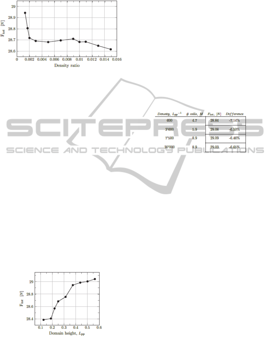
Figure 7: Result of density ratio investigation. The default
value in Shipflow was set to 0.01. The percent decrease
from 0.0013 to 0.01 is 0.90%.
Notice in Figure 7 that the trend is diverging as
the density ratio decreases and goes toward a value
of the physical density ratio of 0.0013. No results
from values below 0.0013 are reported because these
simulations did not converge.
The difference of 0.90% decrease from 0.0013 to
0.01 is not considered insignificant. However, as the
results in the region of low density ratio are
diverging rapidly, these results are not trustworthy
and this quantification shall be viewed with caution.
5.1.2 Domain Height
This investigation was done in order to see the effect
of the height of the domain on the resistance but also
the free water surface geometry in the transom area.
Water on the transom was appearing in the
simulations even though the transom evidently was
clear during the towing tank tests. The height of the
domain here refers to the height of the volume above
the water surface, occupied by air.
The number of cells in the z direction was kept
constant when the domain height was changed. The
results of this investigation can be seen in the
following figure:
Figure 8: Result of domain height investigation, domain
height refers to the height above the static water surface.
Default value in Shipflow was set to 0.5.
Notice in figure 8 that the resulting force increases
rapidly until 0.375 L
pp
. The result from the
investigation shows a decrease by 2.27% from 0.563
to 0.125, with a plateau starting 0.375 L
pp
. Domain
heights over 0.563 L
pp
gave diverging simulations.
5.1.3 Turbulence Models
The selected software Shipflow implements two
turbulence models: SST k-ω and EASM, see section
2.2.2. As the different turbulence models give good
results for different types of flows, both of these
were tested in the validation case. The results are
presented in table 1.
Table 1: Grid dependency points data.
Concluded from this investigation is that the SST
k-ω model is the superior one for this case. The
EASM did not only predict a too-low total
resistance, it also took a lot longer to converge. The
medium-density grid with the EASM converged
with an oscillating trend, and a mean value over
2000 iterations had to be selected. This interval
represented roughly two periods of the oscillating
behaviour. The SST k-ω was then used for the
forthcoming simulations.
5.1.4 Cell Density in the Transom Region
This investigation also originated in having water
creeping up on the vertical transom of the dinghy.
The cause of this water was thought to be an
insufficient resolution of the grid at the corner where
the transom meets the bottom of the hull.
A consequence of refining the grid locally in the
transom area is the grid density at midships.
Stretching functions are used in the meshing tool of
the software, which makes the very fine cells
gradually grow larger with a certain factor. This
makes the cells at midships rather large as a limited
number of cells is used to cover the length between
perpendiculars. This could have been avoided by
adding more cells in this area, but as the transom
was the area of interest in this investigation this was
not done. The longitudinal direction was selected for
refinement. The results of this investigation can be
seen in table2.
icSPORTS2014-InternationalCongressonSportSciencesResearchandTechnologySupport
198
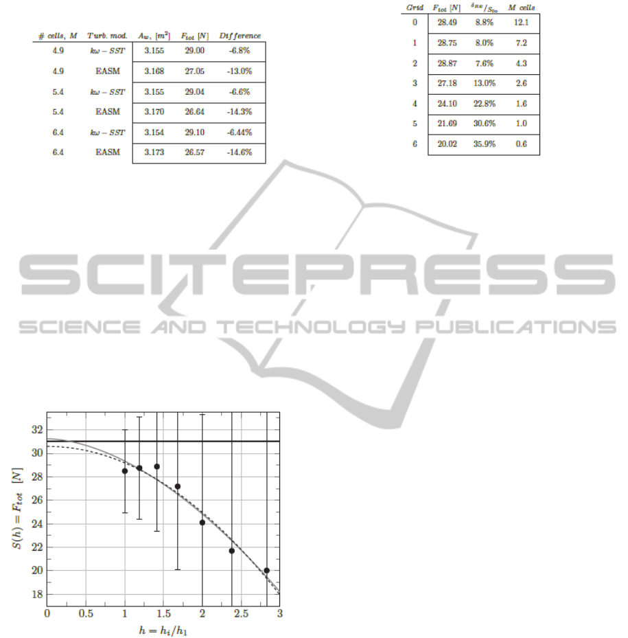
Table 2: Result of the transom grid refinement
investigation. The cell density is in the longitudinal
direction, in the region aft of the transom.
The conclusion of the grid refinement was that
the transom water could be reduced by refining the
transom grid, but it could not be totally cleared.
However, the sought gain in resistance was almost
negligible and the cost for resolving the flow was
significantly increased. This concluded that the
transom grid was not the major cause of the too-low
predicted total resistance.
5.2 Result of the Verification
After selecting the best settings from the numerical
parameter studies, the following verification was
obtained (as shown in figure 9 and table 3):
Figure 9: Grid convergence plot. Gray line = curve fit
obtained order of accuracy; 1.75. Obtained S0 = 31.24N.
Black line = test data; 31.1N.
Evident in this grid-dependence study is that there is
a strong grid dependency. This means that a
substantial increase in grid definition should be able
to eliminate the ~7% error. The problem associated
with a further increase is the lack of memory on the
machines used to run the simulation during this
study. The limit for the available 24GB seemed to be
around 14.5 million cells.
Table 3: Grid dependency points data.
A further refinement of r equal to the 4
th
root of 2
would result in ~20.3 million cells, but a higher
refinement factor is probably needed as there is no
improvement observed for the finest presented grid.
The conclusion of the grid dependence study is
that the grid setup from grid 2 shall be used. To
decide which grid refinement results in a reasonable
error, the result is weighed against the computation
time. As grid 2 gave the best results and did not have
the highest computation time, it was selected.
Grid dependency for an appendage and leeway
case was not done, as the grid settings for the boxed
grid, required to include leeway, were not
successfully changed. This was due to lack of
knowledge in the meshing tool, which led to an
inability to systematically refine the grid.
6 VALIDATION RESULTS AND
DISCUSSION
The main investigation of the paper was to see if the
minima in resistance could be predicted at the same
angles of heel and trim, using the following
methods: bare-hull towing tank tests, bare-hull
simulations and simulations with appendages and
leeway. If this is the case, the more time-consuming
asymmetrical simulations needed for handling the
leeway can be rejected for future investigations of
this kind. The leeway simulations with the
appendages are interesting because they represent
real sailing conditions in the most accurate way
possible in a steady state setup.
The cases that are included in this study are heel
variation for zero trim and the trim variation for zero
heel. To find a global minima in resistance
combinations of heel and trim have to be simulated
as well.
A full series of simulations of heel and trim
variation was not completed. This was thought to be
due to a lack of knowledge in the software, that it is
still a young application of the VOF method and that
CFDPredictionoftheEffectofAppendagesandLeewayontheForceTrendofanOlympicClassLaserDinghyHull
199
it is usually handles ships of a very different kind.
The results of the simulations that are finished are
shown in the following section.
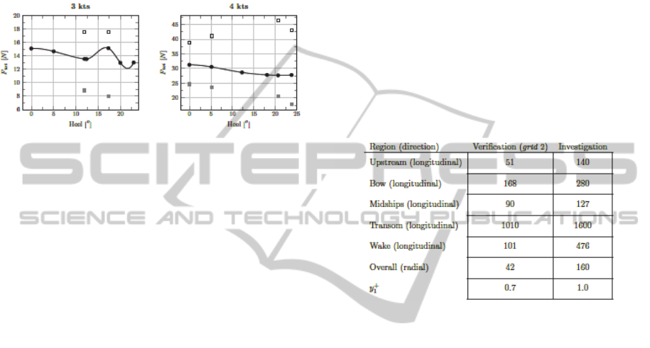
6.1 Heel Variation
The results of the systematic heel variations are
presented in figure 10.
Figure 10: Results of the heel variation. Black = test data,
Gray = bare hull simulations, White = Appendages and
leeway simulations.
The bare-hull simulations that are finished, and
shall be validated against the towing tank test data,
are still predicting very low resistance. This is
despite the use of the selected numerical parameters
from the variation study.
Concluded from the available results from the
four-knots-heel variation for the bare-hull cases is
that the error is larger than the error obtained in the
verification study. The best grid density was then
found to be one containing 4.3 million cells and the
settings for this grid would now be used for all the
simulations during the investigation. The exact grid
settings, however, could not be used, as the grid
layout will be changed. The grid layout used in the
verification study was H-O-grids, explained in
section 3.1. For the investigation part, however, the
boxed and overlapping grid was used. The reason for
this was that the simulations including leeway could
not be done in the H-O-grid. The bare-hull
simulations were also computed using the boxed
grid during the investigation to eliminate the effect
of different grid types on a comparison.
The setup of the boxed grid with the selected
settings was not done successfully. The reason for
this was a lack of knowledge in the meshing tool of
the software. A default setting had to be used
instead, which prevented the specific settings used in
the verification study to be applied.
The default grid settings led to a grid of 7.6
million cells. Recall that this setup is no longer
symmetrical through the centreline, and this would
therefore have corresponded to 3.8 million in the
verification case (where a grid of 4.3 million cells
was preferred). As can be seen in the depiction of
the 4 kts case the bare-hull simulations are some
~20% below the test data. Evaluating the results of
the verification the following fact can be observed;
first, a 20% error would have been predicted for a
grid of only 1.6 million cells, and then for a grid of
3.8 million cells an error of 12.1% could have been
anticipated. This mismatch between results is a
consequence of not being able to use the selected
grid settings. This also means that the errors of any
simulation with the default grid settings cannot be
estimated by the current grid dependence study. The
used cell densities are displayed in table 4.
Table 4: Comparison of cell densities at different regions.
Densities are expressed in cells per Lpp, y is expressed in
the dimensionless length unit.
This means that there are no means of evaluating
the error in these simulations. As there is no
complete series of heel variation, the trends of these
series are not available either, all indicating the need
for further research.
6.2 Trim Variation
The same goes for the trim variations; there are not
enough finished simulations to draw any conclusion.
7 CONCLUDING REMARKS
7.1 Systematic Variation of Numerical
Parameters
This section will sum up the study of systematic
variation of numerical parameters. The study
included four different parameters that were
expected to have an impact on the predicted
resistance of the simulations. These simulations
were conducted on grids of 4.5 to 6.5 million cells,
which turned out to be somewhere at the ~7%
plateau.
Density ratio. The result of this study was that
icSPORTS2014-InternationalCongressonSportSciencesResearchandTechnologySupport
200

the most favorable density ratio was 0.01. The
resistance, however, could be increased by 0.90% by
using the physical density ratio, but as this led to
very numerically unstable simulations this was not
prioritized.
The conclusion of this investigation was that the
results seem to reach a plateau at 0.005 and the fact
that a higher density ratio really did make the
simulations more stable. Also, as only a small
increase in resistance was observed, it was decided
to continue the thesis work with the density ratio set
to 0.01.
Domain height. The domain height had a
significant effect on the resistance but also affected
the numerical stability of the simulation. Changing
the domain height from 0.563 to 0.125 L
pp
resulted
in a decrease of 2.27%. Above 0.536 the simulations
became too numerically unstable. As the domain
height was ~0.5 L
pp
in the previous simulations
already, and the threshold of domain height seemed
to be 0.536, the positive effect of increased domain
height could not be further exploited. The domain
height was therefore kept at 0.5 L
pp
.
Concluded from this investigation was that the
domain height shall be set to 0.5 L
pp
, or in this
particular case 2 meters, in order to still be in the
region of numerical stability but also to give a
resistance as close to the towing tank test result as
possible.
Turbulence models. The turbulence models that
were implemented for the VOF method in the
Shipflow software were EASM and SST k-ω. The
previously used SST k-ω was clearly superior to the
EASM in this case. As the EASM predicted a twice-
as-large error and took substantially more time to
converge, the SST k-ω was selected.
Cell density in the transom region. The
transom region was refined from the previously used
600 cells per L
pp
, to 60’000. Only a slight increase in
resistance, 0.51%, was noticed. This study could
benefit, however, from more thorough investigation,
as it was discovered that cell density in other areas
of the hull was greatly affected by the transom area.
What can be concluded is that an insufficient
resolution in the transom area alone is not a major
source of error.
Some of the cases run during the main
investigation of this study converged to an
oscillating behaviour. This can be due to the fact that
the flow is not steady state after all. If the flow is
unsteady in the transom region, it can result in that
the steady state simulation gives this transom water
as a result. To test if the flow is unsteady, a transient
simulation has to be done, but as the selected
software did not have this option, this was not
investigated.
Another way of obtaining an unsteady flow in
the simulation is if the waves are not small enough
when they are leaving the domain. The remedy for
this will then be to increase the overall size of the
domain in order for the waves to naturally dampen
before reaching the boundaries.
7.2 Investigation
Though no conclusion can be made regarding where
the major source of this ~7% error lies, at least some
numerical parameters can be ruled out by this study,
facilitating further studies in the area.
The study presented in Chapter 5 took most of
the time devoted to this project. As no source for the
error was found during this study, the thesis work
moved on with a modelling setup that was not
accurate. As the objective of this paper is to find a
minima point of a series of heel and trim variations
and not necessarily an absolute value, it was still
considered possible. The setting selected during this
study was to be used in the investigation to the
largest possible extent. All grid density settings were
not to be kept completely similar, as the
investigation would be performed with the boxed
grid setup explained in section 3.1.
As explained in section 5.2, keeping similar grid
settings was not possible at all. The even-keel bare-
hull case was included in the heel and trim variations
but resulted in an even lower resistance than during
the verification. As there were larger errors than
expected by the grid dependence study, the
importance of a good grid became even more
evident. However, as the error for the verification
case increased so dramatically during the
investigation, it can also be concluded that the boxed
grid does not perform equally well in this case. This
conclusion can be made as the verification case was
tested with a non-symmetric H-O-grid as well. The
resistance was then 6.9% less than the towing tank
test run, compared to the 7.6% of the symmetric
case.
To be able to make decisive conclusions, further
investigation needs to be conducted. First of all,
decide if the VOF method should be used, and then
complete the heel and trim variations. The potential
flow method implemented in the software was tested
after this study, on the verification case, and
predicted the resistance within half a percent.
Here follows a list of suggestions for interesting
future research:
Simulate the full test matrix. To see get the
CFDPredictionoftheEffectofAppendagesandLeewayontheForceTrendofanOlympicClassLaserDinghyHull
201

global minima in resistance.
Provide sailing recommendations. Evaluate the
results of the heel and trim variations and make an
instruction of how to achieve highest velocity made
good, including a VPP study.
Investigate actual velocities and attitudes.
Study the sailors to see which velocities and
attitudes are common, to see if there is room for
improvement.
Tailor for individual crew weights. To really
maximize the effect of the individual sailor, a
separate investigation for the weight of the
individual sailor could be performed.
ACKNOWLEDGEMENTS
The authors would like to express their gratitude to
Professor Lars Larsson, Chalmers University of
Technology, Michal Orych, Flowtech International
and Matz Brown, SSPA Sweden AB, for their
contributions to this paper. Further we acknowledge
the financial support provided by Västra
Götalandsregionen, Regionutvecklings-nämnden.
REFERENCES
Davidsson, L., 2003. An Introduction to Turbulence
Models. Chalmers University of technology,
Göteborg.
Deng, Queutey, and Visonneau, 2005. Three dimensional
Flow Computation with Reynolds Stress and
Algebraic Stress Models. Engineering Turbulence
Modelling and Experiments (6), pp: 389-398.
Eca and Hoekstra, 2006. Discretization Uncertainty
Estimation Based on a Least SquaresVersion of the
Grid Convergence Index. In: 2
nd
Workshop on CFD
Uncertainty Analysis; Lisabon; October 2006.
Eca and Hoekstra, 2014. A procedure for the estimation of
the numerical uncertainty of CFD calculations based
on grid renement studies. Journal of Computational
Physics 262, pp: 104-130.
Feymark, A., 2013. A Large Eddy Simulation Based Fluid-
Structure Interaction Methodology with Application in
Hydroelasticity. PhD thesis. Chalmers, Göteborg.
Gatski and Speziale, 1993. On explicit algebraic stress
models for complex turbulent fows. Journal of Fluid
Mechanics (254), pp. 59-78.
Hirt, C. W. and Nichols, B-D., 1979. Volume of Fluid
(VOF) Method for the Dynamics of Free Boundaries.
Los Alamos Scientific Laboratory, New Mexico.
Hirt and Nichols, 1998. Volume of Fluid (VOF) Method
for the Dynamics of Free Boundaries. Journal of
Computaional Physics (39), pp: 201-225.
Larsson and Raven, 2010. Ship Resistance and Flow. The
Society of Naval Architects and Marine Engineers.
Marek, Aniszewski and Boguslawski, 2008. Simplified
Volume of Fluid Method (SVOF) for Two-Phase
Flows. Czestochowa University of Technology,
Poland.
Menter, F. R., 1994. Two-equation eddy-viscosity
turbulence models for engineering applications. AIAA
Journal, Vol. 32, No. 8, pp: 1598-1605.
Orych, Larsson, and Regnstrom, 2010. Adaptive
overlapping grid techniques and spatial discretization
schemes for increasing surface sharpness and
numerical accuracy in free surface capturing methods.
28
th
Symposium on Naval Hydrodynamics, Pasadena
California, pp: 389-398.
Roache, P., 1998. Verication and Validation in
Computational Science and Engineering. Hermosa
Publishers.
Roy, C., 2003. Grid Convergence Error Analysis for
Mixed-Order Numerical Schemes. The American
Institute of Aeronautics and Astronautics (41), pp:
596-604.
Rumsey, C., 2013. The Menter Shear Stress Transport
Turbulence Model. Web Article.
url: http://turbmodels.larc.nasa.gov/sst.html.
Slater, J. W., 2005. Examining Spatial Grid Convergence.
Web Article. 2005.
url: http://grc.nasa.gov/WWW/wind/valid/tutorial/
spatconv.html.
Versteeg and Malalasekera, 2007. An Introduction.
to Computational Fluid Dynamics: The Finite Volume
Method (2nd Edition). Prentice Hall.
Wallin, S. and Johansson, A. V., 2000. An Explicit
Algebraic Reynolds Stress Model for Incompressible
and Compressible Turbulent Flows. Fluid Mechanics,
Vol. 403, pp: 89-132.
Zou and Larsson, 2010. A Verication and Validation Study
Based on Resistance Submissions. In: Numerical Ship
Hydrodynamics 2010. Workshop, pp: 203-254.
icSPORTS2014-InternationalCongressonSportSciencesResearchandTechnologySupport
202
