
Maximum Message Flow and Capacity
in Sensor Networks
Vassil S. Sgurev, Stanislav T. Drangajov, and Lyubka A. Doukovska
Institute of Information and Communication Technologies, Bulgarian Academy of Sciences
Acad. G. Bonchev str., bl. 2, 1113 Sofia, Bulgaria
vsgurev@gmail.com; sdrangajov@gmail.com, doukovska@iit.bas.bg
Keywords: Sensors, Receivers, Communication network, Network flow optimization methods.
Abstract: The present paper considers problems for defining of the maximal messages traffic in a communication
network with limited capacities of the separate sections and with arbitrary location of sensors and receivers
on it. The specific requirements are described which emerge from the operation of the sensors and receivers
on the communication network. Network flow methods are proposed for calculating the maximum possible
messages flow, including such a flow of min cost, as well as of the set of critical sections of the network,
which block the possibility of further increase of the messages flow. These methods take in account the
specific features at generating and receiving of information by the sensors and the receivers respectively.
Two numerical examples are given which practically illustrate the solving of the problems pointed out
above, and show the effectiveness of the methods proposed for modelling and optimization.
1 PRELIMINARY
Many areas of science and technologies exist where
machines and apparatuses are used, equipped with
multiple sensors and receivers for the signals and
messages, emitted by the former. All of them are
connected in sophisticated communication networks
for information transfer and distribution; as such
may be considered the different centers for physical
experiments, machines and equipment in the energy
industry – from solar plates to heavy oil sea stations,
nuclear electrical power plants, transportation
systems, and so on. In fact no area – production,
social, or economical – exists where the information
flows are not of great importance and as so the speed
and reliability of the connections should be by no
means neglected. This is of course directly connected
with the tremendous flourish of information techno-
logies, which propose possibilities for information
flows control.
The network flow programming methods and
algorithms (Ford, Fulkerson, 1956) propose a good
ground for investigation and realization of the
message planning and routing. These methods and
algorithms, though a particular class of mathematical
programming, turn to be very effective and quickly
convergent (Shakkottai, Srikant, 2007; Sgurev, 1991).
2 THE SENSOR
COMMUNICATION NETWORK
It is most convenient to represent the sensors
communication network as an oriented graph
G(X, U) (Christofides, 1986) with a set of arcs U and
a set of noes X, such that:
;),( ;
),(
Gji
ii
Ii
i
xxUxX
(1)
;)( ;)(
rts
IIIIRTSX
(2)
; ; ;
rts
Ii
i
Ii
i
Ii
i
xRxTxS
(3)
where S is the set of sensor points; T – the set
of information receiver points; R – the set of inter-
mediate points through the information is being
transported without any processing; A – the set
of pairs of indices of all arcs from U such that
A = {(i, j) / (x
i
, x
j
) U}; x
ij
– brief denotation of the
arc (x
i
, x
j
); Ø – the empty set; I – the set of indices of
all nodes from X; I
s
, I
t
, and I
r
– subsets of indices of
nodes from S, T, and R respectively, for which it is
supposed that:
74
Sgurev V., T. Drangajov S. and Doukovska L.
Maximum Message Flow and Capacity in Sensor Networks.
DOI: 10.5220/0005421500740080
In Proceedings of the Third International Conference on Telecommunications and Remote Sensing (ICTRS 2014), pages 74-80
ISBN: 978-989-758-033-8
Copyright
c
2014 by SCITEPRESS – Science and Technology Publications, Lda. All rights reserved

I
s
∩ I
r
= Ø; I
s
∩ I
t
= Ø; I
r
∩ I
t
= Ø (4)
The direct and reverse mapping on the indices I
on the graph G(X, U) may be represented in the
following way (Christofides, 1986):
};),/({
1
XxUxxj
jjii
(5)
};),/({
1
XxUxxj
jiji
(6)
It is expedient the discrete messages from the
separate sensors and for a given time gap Δt to be
averaged by number and duration. This will allow
them to be considered as a continuous flow of
messages with an average statistical flow density
(Sgurev, 1991), from one point to another.
If a possibility exists for simultaneous trans-
mission of messages from x
i
to x
j
and vice versa,
then the respective section (x
i
, x
j
) is replaced
by a pair of oppositely directed arcs and namely
{(x
i
, x
j
), (x
j
, x
i
)}
U.
The average statistical density of the message
flow being emitted from the sensor of index i I
may be defined in the following way:
; ;
s
Dp
ip
i
Ii
t
f
i
(7)
where
ip
– duration of the k
-th
in order message from
the sensor i I
s
; D
i
– the set of indices of the
messages received from the sensor of index i I
s
in
the time gap Δt.
For the receiver points with indices from It this
value will look like this:
; ;
t
Hk
jp
j
Ij
t
f
j
(8)
where
jp
is the duration of the k
-th
in order
message to the receiver of index j I
t
; H
j
– the set
of indices of messages received by point j.
If we proceed from the assumption that no loss of
messages is admissible at their transportation through
the network, then equality is necessary between the
sum of the densities of the messages emitted by all
sensors of indices from I
s
and the sum of densities of
the messages, received by all receivers with indices
from I
t
, i.e.:
;v
j
f
i
f
t
Ij
s
Ii
(9)
where v is the total density of all messages being
transferred from all sensors to all receivers.
In most cases the increase or decrease of the flow
density from any sensor of index i I
s
and to any
receiver of index j I
t
is proportional to their
inherent technical characteristics defined by the
parameters f
i
and f
j
from (7) and (8) respectively. It
follows then from (9) that for each i I
s
and j I
t
the following coefficients could be calculated:
; ; vkf
v
f
f
f
k
ii
i
Ii
i
i
i
s
(10)
. ; vkf
v
f
f
f
k
jj
j
Ii
j
j
j
s
(11)
If both sides of the equalities (10) and (11) are
summed on i I
s
and j I
t
respectively, then:
.1
t
Ij
s
Ii
j
k
i
k
(12)
The density of the message flow from x
i
to x
j
will
be denoted by the arc flow function f
ij
; (i, j) A and
by c
ij
; (i, j) A will be denoted the capacity of the
arc x
ij
. Then the next requirement shows the physical
impossibility the flow function density f
ij
to exceed
the capacity c
ij
of the arc x
ij
, i.e. for each (i, j) A:
0 ≤ f
ij
≤ c
ij
(13)
The value of a unit of density of the messages
flow will be denoted by the non-negative arc rate
a
ij
≥ 0; (i, j) A on the respective arc (section) x
ij
.
The following two important problems may be
formulated on the sensor communication networks:
A. Find the maximum possible flow v
max
from the
sensor points S to receiver points T. This may be
most effectively performed through the following
network programming problem:
L = v → max (14)
subject to the following constraints, for each i I:
; if ,
; if ,0
; if ,
11
ti
r
si
j
ji
j
ij
Iik
Ii
Iivk
ff
ii
(15)
Maximum Message Flow and Capacity in Sensor Networks
75

f
ij
≤ c
ij
, for each (i,j) ϵ A (16)
f
ij
≥ 0, for each (i,j) ϵ A (17)
Solving the problem above results in:
L = v
max
(18)
Let cuts
)(
0,0
XX
be defined between S and T as sets
of arcs, such that:
X
0
X; (19)
; ;\
0000
XXXXX
};;/{),(
0000
UxXXXxxXX
ijjiij
(20)
Then, according to the well-known min-cut max-
flow theorem of Ford-Fulkerson (Ford, Fulkerson,
1956) a minimal cut
),(
*
0
*
0
XX
is the one for which:
0),();,(),(
*
0
*
0
*
0
*
0
*
0
*
0
XXfXXcXXf
(21)
It follows then that the max flow value may be
increased only if the capacity of some arcs of the
minimal cut
),(
*
0
*
0
XXx
ij
is increased. Further on the
arcs with equality between the capacity and the arc
flow function will be called saturated and otherwise
– unsaturated.
B. As it is possible several minimal cuts to exist the
problem arises to find the one of them which is of
minimal value of the parameter
Aji
ijij
fa
),(
. For
solving this problem it is necessary problem A. to be
first solved, i.e. the max flow v
max
from (18) to be
found through relations (14) to (17) and then with
fixed max flow the minimal cut of minimal cost to be
defined. For this purpose the values of {k
i
v / i I
s
}
and {k
j
v / j I
t
} are calculated with known v = v
max
and the latter to be put down as fixed values in the
right hand side of (15). Then finding of the minimal
cut of minimal cost may be carried out by solving the
following network flow programming problem:
Aji
ijij
faL
),(
min
(22)
observing constraints (14) to (17).
This method provides a possibility for optimal
distribution (max flow and min cost) of the messages
traffic between the sensors and the receivers in the
sensor communication network.
3 EXEMPLARY PROBLEM AND
NUMERICAL SOLUTIONS
The numerical examples which follow demonstrate
the abilities of the method proposed for finding the
maximal flow from the sensors to receivers (Problem
A.) and the minimal cut with minimal cost (Problem
B.).
EXAMPLE: A sensor communication network with
9 nodes and 17 arcs (sections) is conditionally shown
in Figure 1.
Three nodes are sensors, 3 – receivers, and 3 –
intermediate, and namely:
S = {x
1
, x
2
, x
3
}; T = {x
7
, x
8
, x
9
}; R = {x
4
, x
5
, x
6
}.
The oriented arcs in Figure 1 show from which
initial node to which final node messages are being
transmitted. The capacities {c
ij
} and the rates {a
ij
}
for each arc of the network are shown in Table 1.
The messages densities from sensors S to receiver
points T are put down in Table 2. In the same table
the values of coefficients {k
i
} and {k
j
} are given,
calculated according to formulae (10) and (11).
Table 1: Capacities and Rates
A
(1,2)
(1,4)
(1,5)
(1,7)
(2,3)
(2,4)
(3,4)
(3,6)
(3,9)
(4,5)
(4,6)
(5,7)
(5,8)
(6,8)
(6,9)
(8,7)
(9,8)
c
ij
5
3
7
6
7
6
6
9
4
8
5
7
8
6
11
5
6
a
ij
10
5
5
10
11
6
6
5
10
5
5
3
4
7
4
6
10
Third International Conference on Telecommunications and Remote Sensing
76
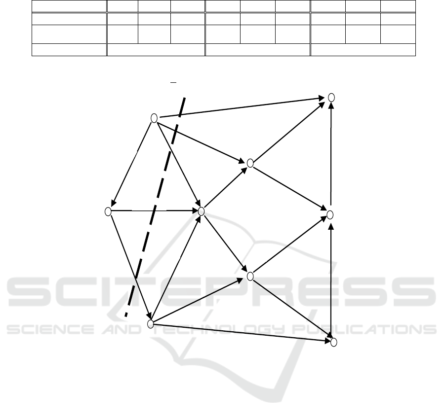
Table 2: Coefficients {k
i
} and {k
j
}
Nodes X
x
1
x
2
x
3
x
4
x
5
x
6
x
7
x
8
x
9
{f
i
}
14
10
6
0
0
0
9
9
12
{k
i
}
{
j
k
}
0,47
0,33
0,2
-
-
-
0,3
0,3
0,4
Node type
Sensor
Intermediate
Receiver
),(
00
XX
Fig. 1. A sensor communication network with 9 nodes and 17 arcs
x
1
6(6)
x
7
1
1,04
(5)
x
5
x
2
x
8
6(6)
1,2
5(6)
7(7))
4,875(7)
x
4
3(3)
5(5)
8(8)
9(9)
3(6)
x
6
1
7(7)
x
3
x
9
0,5(6)
4(4)
0(5)
11(11)
5,25(8)
Figure 1: A sensor communication network with 8 nodes and 17 arcs
A. On the base of the data from Tables 1 and 2 the
problem for finding the maximal flow v
max
may be
reduced to the following problem of network flow
programming. Maximization of v from the linear
form (14) observing the following equalities and
inequalities:
z
1
) f
1,2
+ f
1,4
+ f
1,5
+ f
1,7
= 0,47 v; z
2
) f
2,3
+ f
2,4
- f
1,2
= 0,33 v;
z
3
) f
3,4
+ f
3,6
+ f
3,9
+ f
2,3
= 0,2 v ; z
4
) f
4,5
+ f
4,6
- f
1,4
- f
2,4
- f
3,4
= 0;
z
5
) f
5,7
+ f
5,8
- f
1,5
- f
4,5
= 0; z
6
) f
6,8
+ f
6,9
- f
3,6
- f
4,6
= 0;
z
7
) f
1,7
+ f
5,7
+- f
8,7
= 0,3 v; z
8
) f
5,8
+ f
6,8
+ f
9,8
- f
8,7
= 0,3 v;
z
9
) f
3,9
+ f
6,9
- f
9,8
= 0,4 v;
z
10
) f
1,2
≤ 5; z
11
) f
1,4
≤ 3 z
12
) f
1,5
≤ 7;
z
13
) f
1,7
≤ 6; z
14
) f
2,3
≤ 7 z
15
) f
2,4
≤ 6;
z
16
) f
3,4
≤ 6; z
17
) f
3,6
≤ 9 z
18
) f
3,9
≤ 4;
z
19
) f
4,5
≤ 8; z
20
) f
4,6
≤ 5 z
21
) f
5,7
≤ 7;
z
22
) f
5,8
≤ 8; z
23
) f
6,8
≤ 6 z
24
) f
6,9
≤ 11;
z
25
) f
8,7
≤ 5; z
26
) f
9,8
≤ 6 z
27
) f
i,j
≥ 0 for each (i, j) A.
Maximum Message Flow and Capacity in Sensor Networks
77

Table 3: Arc flow function density
Arc flow
density f
i,j
f
1,2
f
1,4
f
1,5
f
1,7
f
2,3
f
2,4
f
3,4
f
3,6
f
3,9
f
4,5
f
4,6
f
5,7
f
5,8
f
6,8
f
6,9
f
8,7
f
9,8
Value
1,04
3
7
6
7
6
1,25
9
4
5,25
5
4,875
7,375
3
11
0
0,5
The problem described above was solved by the
software product WebOptim (Genova et al., 2011).
The results obtained are summarized in the next
Table 3 with value of v
max
= 36,25.
If data above for {f
ij
} are used and also the arc
rates {a
ij
} from Table 1, then the costs for messages
transportation, corresponding to the maximal flow
defined above, and namely:
Aji
ijij
fa
),(
25,491
(23)
On the base of the coefficients {k
i
} and {k
j
}
from Table 2 and the maximal flow achieved
v
max
= 36,25 the maximum admissible flow densities
of messages may be calculated from the sensors S to
the receiver points T, i.e.:
k
1
v = 17,04; k
2
v = 11,96; k
3
v = 7,25 (24)
875,10
7
vk
;
875,10
8
vk
;
50,14
9
vk
(25)
On each arc in Figure 1 its main parameters are
shown – the arc flow function, and in brackets the
arc capacity. On the same figure the cut is shown by
thick dotted line
),(
00
XX
= {x
14
, x
15
, x
17
, x
23
, x
24
}
for which there is equality between the maximal
possible flow and the minimal cut, i.e. for which
requirements (21) are observed. Node x
3
cannot be
added to the nodes X
0
= {x
1
, x
2
} of this cut
),(
00
XX
because its parameter k
3
v is linearly related to k
1
v
and k
2
v which are blocked by the minimal cut
),(
00
XX
. Therefore k
3
v cannot be increased
although that a path exists from it {x
34
, x
45
, x
57
} to
the receiver point x
7
with unsaturated arcs. This is a
specific feature of the sensor communication
networks reflected in (10) and (11) which does not
allow Ford-Fulkeson theorem to be directly applied,
but in an oblique way only. In case that increase of
the flow v is needed from S to T this should be
performed by increasing the capacity of an arc from
the cut:
),(
00
XX
= {x
14
, x
15
, x
17
, x
23
, x
24
} (26)
B. For calculating the maximal flow of minimal cost
relations z
1
to z
27
with the following changes:
the right hand sides of equations z
1
to z
3
are
replaced by the respective right hand parts of
the three relations from (25);
the right hand sides of equations z
7
to z
9
are
replaced by the respective right hand parts of
the three relations from (26). In this way the
maximal possible flow v
max
is fixed both in the
sensors S and in the receivers T.
For finding the minimal value of this flow the
following linear relation is used in thich the rates
{a
ij
} are taken from Table 1:
L
1
= 10 f
1,2
+ 5 f
1,4
+ 5 f
1,5
+ 10 f
1,7
+ 11 f
2,3
+ 6 f
2,4
+ 6
f
3,4
+ 5 f
3,6
+ 10 f
3,9
+ 5 f
4,5
+ 5 f
4,6
+ 3 f
5,7
+ 4 f
5,8
+ 7 f
6,8
+ 4 f
6,9
+ 6 f
8,7
+ 10 f
9,8
→ min (27)
The problem (27) with the modified relations z
1
to z
27
was solved by the software product mentioned
above. The values of the arc flow functions and of
the linear form (27) are summarized in the Table 4:
L
1
= 485,53 (28)
Table 4: Arc Flow Function
Arc flow
function f
i,j
f
1,2
f
1,4
f
1,5
f
1,7
f
2,3
f
2,4
f
3,4
f
3,6
f
3,9
f
4,5
f
4,6
f
5,7
f
5,8
f
6,8
f
6,9
f
8,7
f
9,8
Value
1,03
3
7
6
7
6
1,24
9
4
5,87
4,37
4,87
8
2,87
10,5
0
0
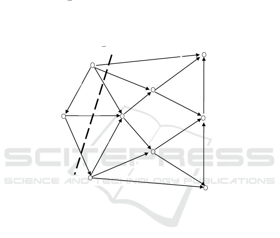
These data are put down in the Figure 2 like in
Figure 1. In both numerical examples – in case A
(Figure 1) and in case B (Figure 2) the configuration
of the graph G(X,U), capacities {c
ij
}, coefficients {k
i
}
and {k
j
}, arc rates {a
ij
} and the max flow v
max
are
identical but there is a difference in the flow
realization of {f
ij
}. The flow value on the arc x
4,5
in
case A is 5,25 and in case B – 5,87. There are
Third International Conference on Telecommunications and Remote Sensing
78
changes and on the arcs {x
4,6
, x
5,7
, x
5,8
, x
6,8
, x
6,9
, x
8,9
}.
Some of them (x
4,6
, x
6,9
) has turned from saturated
into unsaturated ones, another one (x
5,8
) – from
unsaturated into saturated, and third – (x
4,6
, x
5,7
, x
6,8
,
x
8,9
), has only changed the flow function values.
The minimal cut
),(
00
XX
; X
0
= {x
1
, x
2
} remains
the same as in Figure 1 and due to the same reasons it
blocks the maximal flow increase. If the total value
of the maximum possible traffic in both cases – A
and B, then as expected from (23) and (29) for the
max flow of min cost the total value L
1
is less by
about 1,2% less than the analogical value L
corresponding to the first case, i.e.:
ΔL = L – L
1
= 491,25 – 485,53 = 5,72 (29)
The two examples given in the cases A and B
demonstrate the effectiveness of the method pro-
posed for finding of the maximum messages flow
from sensor to receiver points on an arbitrary sensor
communication network, and of max flow of min
cost.
),(
00
XX
Fig. 2. The same network with optimal values
x
1
6(6)
x
7
1
1,04
(5)
x
5
x
2
x
8
6(6)
1,2
5(6)
7(7)
4,87(7)
x
4
3(3)
4,37
(5)
8(8)
9(9)
2,87(6)
x
6
1
7(7)
x
3
x
9
0(6)
4(4)
0(5)
10,5(11)
5,87(8)
Figure 2: The same network with optimal values
4 SUMMARY
Here we show that the graph theory and network
flow methods and algorithms are still up-to-date for
control and optimization of the ‘commodity’ traffic
in our case – messages from sensors to receivers,
ensuring max flow at min cost of the traffic across
the network. Two approaches are proposed for
sensor networks, which maximize the flow from
sensors to receivers and minimize the cost of this
flow. In the first one the max flow is found and in
the second one – alternative paths of min cost are
found. The advantage of the network flow
optimization is that it is independent on the nature
and the physical characteristics of the network and
operates with abstract and relative quantities, which
when scaled in appropriate way are applicable to any
type of real networks.
ACKNOWLEDGEMENTS
The research in the paper is partly supported by the
project AComIn “Advanced Computing for
Innovation”, Grant 316087, funded by the FP7
Capacity Programme (Research Potential of
Convergence Regions) and partly supported under the
Project № DVU-10-0267/10.
Maximum Message Flow and Capacity in Sensor Networks
79

REFERENCES
Sgurev V., 1991. Network Flows with General
Constraints, Publishing House of the Bulgarian
Academy of Sciences, Sofia (in Bulgarian).
Christofides N., 1986. Graph Theory: An
Algorithmic Approach, London: Academic Press.
Shakkottai S., R. Srikant, 2007. Network
Optimization and Control. Foundations and
Trends in Networking, Vol. 2, № 3, pp. 271–379.
Ford L. R., D. R. Fulkerson, 1956. Maximal flow
through a network. Canadian Journal of
Mathematics, Vol. 8, pp. 399–404.
Bertsecas D., 1991. Linear Network Optimization,
Massachusetts Institute of Technology.
Jensen P., J. Barnes, 1980. Network Flow Program-
ming, John Wiley & Sons, NY, USA.
Genova K., L. Kirilov, V. Guliashki, B. Staykov, D.
Vatov, 2011. A Prototype of a Web-based
Decision Support, System for Building Models
and Solving Optimization and Decision Making
Problems, In: Proceedings of XII International
Conference on Computer Systems and
Technologies (Eds. B. Rachev, A. Smrikarov),
Wien, Austria, 16-17 June 2011, ACM ICPS,
Vol. 578, pp. 167–172.
Third International Conference on Telecommunications and Remote Sensing
80
