Intercriteria Decision Making Approach to EU Member States
Competitiveness Analysis
Vassia K. Atanassova
1
, Lyubka A. Doukovska
1
, Krassimir T. Atanassov
2,3
and Deyan G. Mavrov
3
1
Institute of Information and Communication Technologies, Bulgarian Academy of Sciences,
Acad. G. Bonchev str., bl. 2, 1113 Sofia, Bulgaria
2
Institute of Biophysics and Biomedical Engineering, Bulgarian Academy of Sciences,
Acad. G. Bonchev str., bl. 105, 1113 Sofia, Bulgaria
3
Prof. Dr. Asen Zlatarov University, 1 Prof. Yakimov Blvd., 8010 Burgas, Bulgaria
Keywords: Global Competitiveness Index, Index Matrix, Intercriteria Decision Making, Intuitionistic Fuzzy Sets,
Multicriteria Decision Making.
Abstract: In this paper, we present some interesting results derived from the application of our recently developed
decision making approach to data from the World Economic Forum’s Global Competitiveness Reports for
the years 2008–2009 to 2013–2014. The discussed approach, called ‘Intercriteria Decision Making’,
employs the apparatus of index matrices and intuitionistic fuzzy sets to produce from an existing multiobject
multicriteria evaluation table a new table that contains estimations of the pairwise correlations among the set
of evaluating criteria, called ‘pillars of competitiveness’. Using the described approach over the data about
WEF evaluations of the state of competitiveness of the 28 present EU Member States, certain dependences
are discovered to connect the 12 ‘pillars’, termed a ‘positive’ and a ‘negative consonance’. The whole
research and the conclusions derived are in line with WEF’s address to state policy makers to identify and
strengthen the transformative forces that will drive future economic growth.
1 INTRODUCTION
The present work contains a novel analysis of the
most recent Global Competitiveness Reports (GCRs)
of the World Economic Forum (WEF), produced
from 2008–2009 to 2013–2014, aiming at the
discovery of some hidden patterns and trends in the
present Member States of the European Union. We
use a recently developed method, based on
intuitionistic fuzzy sets and index matrices, two
mathematical formalisms proposed and significantly
researched by Atanassov in a series of publications
from 1980s to present day.
The developed method for multicriteria decision
making (Atanassov et al., 2013) is specifically
applicable to situations where some of the criteria
come at a higher cost than others, for instance are
harder, more expensive and/or more time consuming
to measure or evaluate. Such criteria are generally
considered unfavourable, hence if the method
identifies certain level of correlation between such
unfavourable criteria and others that are easier,
cheaper or quicker to measure or evaluate these
might be disregarded in the further decision making
process. In particular, the approach has been so far
applied to petrochemical industry, where the aim has
been to reduce some of the most costly and time
consuming checks of the probes of raw mineral oil,
which have proven to correlate with other cheaper
and quicker tests, thus reducing production costs and
time needed for business decision making.
The present work is the first application of the
developed approach in the field of economics. We
have considered it appropriate to analyse our
selection of data, in order to discover which of the
twelve pillars (criteria) in the formation of the
Global Competitiveness Index (GCI) tend to
correlate. In comparison with related applications of
the method, here, we do not conclude that any of the
correlating criteria might be skipped, as in the
petrochemical case study. We are interested however
to discover dependences between the pillars, which
could help policy makers, especially in the low
performing EU Member States, to focus their efforts
in fewer directions and reasonably expect on the
basis of this analysis that improved country’s
289
Atanassova V., Doukovska L., T. Atanassov K. and Mavrov D.
Intercriteria Decision Making Approach to EU Member States Competitiveness Analysis.
DOI: 10.5220/0005427302890294
In Proceedings of the Fourth International Symposium on Business Modeling and Software Design (BMSD 2014), pages 289-294
ISBN: 978-989-758-032-1
Copyright
c
 2014 by SCITEPRESS – Science and Technology Publications, Lda. All rights reserved

performance against those pillars would positively
affect the performance in the respective correlating
pillars. Such correlation can be deemed reasonable
to expect, as the twelve pillars are based on a
multitude of indicators, some of which enter the GCI
in two difference pillars each, as explained in the
GCR’s Appendix “Computation and structure of the
Global Competitiveness Index” (and to avoid double
counting, half-weight is being assigned to each
instance).
This attempt to identify the correlations between
the different pillars of competitiveness reflects WEF
addressing the countries’ policy makers with the
advice to ‘identify and strengthen the transformative
forces that will drive future economic growth’, as
formulated in the Preface of the latest Global
Competitiveness Report 2013–2014.
This paper is organized as follows. In Section 2
are briefly presented the two basic mathematical
concepts that we use, namely, intuitionistic fuzzy
sets and index matrices. On this basis, the proposed
method is outlined. Section 3 contains our results
from applying the method to analysis of a selection
of data about the performance of the currently 28
Member States of the EU during the last six years
against the twelve pillars of competitiveness. We
report of the findings, produced by the algorithm and
formulate our conclusions in the last Section 4.
2 BASIC CONCEPTS
AND METHOD
The presented multicriteria decision making method
is based on two fundamental concepts: intuitionistic
fuzzy sets and index matrices. It bears the specific
name ‘intercriteria decision making’.
Intuitionistic fuzzy sets defined by Atanassov
(Atanassov, 1983; Atanassov, 1986; Atanassov,
1999; Atanassov, 2012) represent an extension of
the concept of fuzzy sets, as defined by Zadeh
(Zadeh, 1965), exhibiting function µ
A
(x) defining the
membership of an element x to the set A, evaluated
in the [0; 1]-interval. The difference between fuzzy
sets and intuitionistic fuzzy sets (IFSs) is in the
presence of a second function ν
A
(x) defining the non-
membership of the element x to the set A, where:
0 ≤ µ
A
(x) ≤ 1,
0 ≤ ν
A
(x) ≤ 1,
0 ≤ µ
A
(x) + ν
A
(x) ≤ 1.
The IFS itself is formally denoted by:
A = {x, µ
A
(x), ν
A
(x) | x  E}.
Comparison between elements of any two IFSs, say
A and B, involves pairwise comparisons between
their respective elements’ degrees of membership
and non-membership to both sets.
The second concept on which the proposed
method relies is the concept of index matrix, a mat-
rix which features two index sets. The theory behind
the index matrices is described in (Atanassov, 1991).
Here we will start with the index matrix M with
index sets with m rows {C
1
, …, C
m
} and n columns
{O
1
, …, O
n
}:
11 1 1 1
1
1
1
1
1, , , ,
,, ,,
,, ,,
,, ,,
,
kln
iikilin
jjkjljn
mmjmlmn
kln
CO CO CO CO
iCOCO COCO
jCOCO COCO
mCO CO CO CO
OO OO
M
Ca a a a
Ca a a a
Ca a a a
Ca a a a









where for every p, q (1 ≤ p ≤ m, 1 ≤ q ≤ n), C
p
is a
criterion (in our case, one of the twelve pillars), O
q
in an evaluated object (in our case, one of the 28 EU
Member states), a
C
p
O
q
is the evaluation of the q-th
object against the p-th criterion, and it is defined as a
real number or another object that is comparable
according to relation R with all the rest elements of
the index matrix M, so that for each i, j, k it holds the
relation R(a
C
k
O
i
, a
C
k
O
j
). The relation R has dual re-
lation
R
, which is true in the cases when relation R
is false, and vice versa.
For the needs of our decision making method,
pairwise comparisons between every two different
criteria are made along all evaluated objects. During
the comparison, it is maintained one counter of the
number of times when the relation R holds, and
another counter for the dual relation.
Let
,kl
S

be the number of cases in which the rel-
ations R(a
C
k
O
i
, a
C
k
O
j
) and R(a
C
l
O
i
, a
C
l
O
j
) are simul-
taneously satisfied. Let also
,kl
S

be the number of
cases in which the relations R(a
C
k
O
i
, a
C
k
O
j
) and its
dual
R
(a
C
l
O
i
, a
C
l
O
j
) are simultaneously satisfied. As
the total number of pairwise comparisons between
the object is n(n – 1)/2, it is seen that there hold the
inequalities:
,,
(1)
0
2
kl kl
nn
SS



.
Fourth International Symposium on Business Modeling and Software Design
290

For every k, l, such that 1 ≤ k ≤ l ≤ m, and for
n ≥ 2 two numbers are defined:
,,
,,
2, 2
(1) (1)
kl kl
kl kl
CC CC
SS
nn nn

 

.
The pair constructed from these two numbers plays
the role of the intuitionistic fuzzy evaluation of the
relations that can be established between any two
criteria C
k
and C
l
. In this way the index matrix M
that relates evaluated objects with evaluating criteria
can be transformed to another index matrix M* that
gives the relations among the criteria:
11 11 1 1
11
1
1,C,C ,C,C
,C ,C ,C ,C
*
.
,,
,,
mm
m m mm mm
m
CC C C
mCC C C
CC
M
C
C
  
  





The final step of the algorithm is to determine the
degrees of correlation between the criteria,
depending on the user’s choice of µ and ν. We call
these correlations between the criteria: ‘positive
consonance’, ‘negative consonance’ or ‘dissonance’.
Let α, β [0; 1] be given, so that α + β ≤ 1. We
call that criteria C
k
and C
l
are in:
 (α, β)-positive consonance, if µ
C
k
,C
l
> α and ν
C
k
,C
l
< β
;
 (α, β)-negative consonance, if µ
C
k
,C
l
< β and ν
C
k
,C
l
> α
;
 (α, β)-dissonance, otherwise.
Obviously, the larger α and/or the smaller β, the
less number of criteria may be simultaneously
connected with the relation of (α, β)-positive con-
sonance. For practical purposes, it carries the most
information when either the positive or the negative
consonance is as large as possible, while the cases of
dissonance are less informative and can be skipped.
3 MAIN RESULTS
We ran the described algorithm over collected data
from six WEF GCRs for the 28 (current) EU
Member States. Here, we present only the results
from the two extreme periods: years 2008–2009 and
year 2013–2014, comparing them for µ
C
i
C
j
and ν
C
i
C
j
in Tables 1–2. Despite having the results with
precision of 9 digits after the decimal point, we will
use precision of 3 digits after the decimal point.
In Tables 1 and 2, all cells are coloured in the
greyscale, with the highest values coloured in the
darkest shade of grey, while the lowest ones are
coloured in white. Of course, every criteria perfectly
correlates with itself, so for any i the value
µ
C
i
C
i
is
always 1, and
ν
C
i
C
i
= π
C
i
C
i
= 0. Also, the matrices are
obviously symmetrical according to the main dia-
gonal. The twelve pillars are: 1. Institutions; 2. Infra-
structure; 3. Macroeconomic stability; 4. Health and
primary education; 5. Higher education and training;
6. Goods market efficiency; 7. Labour market effic-
iency; 8. Financial market sophistication; 9. Techno-
logical readiness; 10. Market size; 11. Business
sophistication; 12. Innovation.
In the beginning, let us present in Table 3 some
findings from the analysis of the six periods.
Table 1: Comparison of the calculated values of µ
C
i
C
j
for years 2008–2009 and 2013–2014.
µ
1 2 3 4 5 6
7 8 9 10
11
12
1 1.000 0.844 0.685 0.757 0.788 0.833 0.603 0.828 0.823 0.497
0.794
0.802
2 0.844 1.000 0.627 0.751 0.749 0.743 0.529 0.741 0.775 0.582
0.831
0.807
3 0.685 0.627 1.000 0.616 0.638 0.664 0.653 0.648 0.693 0.434
0.651
0.667
4 0.757 0.751 0.616 1.000 0.780 0.720 0.550 0.704 0.725 0.524
0.765
0.772
5 0.788 0.749 0.638 0.780 1.000 0.746 0.622 0.728 0.757 0.558
0.767
0.796
6 0.833 0.743 0.664 0.720 0.746 1.000 0.627 0.817 0.802 0.505
0.786
0.765
7 0.603 0.529 0.653 0.550 0.622 0.627 1.000 0.664 0.611 0.389
0.563
0.590
8 0.828 0.741 0.648 0.704 0.728 0.817 0.664 1.000 0.820 0.476
0.733
0.751
9 0.823 0.775 0.693 0.725 0.757 0.802 0.611 0.820 1.000 0.548
0.817
0.815
10 0.497 0.582 0.434 0.524 0.558 0.505 0.389 0.476 0.548 1.000
0.648
0.601
11 0.794 0.831 0.651 0.765 0.767 0.786 0.563 0.733 0.817 0.648
1.000
0.860
12 0.802 0.807 0.667 0.772 0.796 0.765 0.590 0.751 0.815 0.601
0.860
1.000
µ
1
2
3
4
5
6
7 8 9 10 11
12
1 1.000
0.735 0.577
0.720 0.807 0.836
0.733 0.749 0.854 0.503 0.804 0.844
2 0.735
1.000 0.479
0.661 0.749 0.677
0.537 0.590 0.786 0.661 0.804 0.799
3 0.577
0.479 1.000
0.421 0.519 0.558
0.627 0.675 0.550 0.413 0.548 0.556
4 0.720
0.661 0.421
1.000 0.730 0.683
0.590 0.563 0.677 0.497 0.712 0.690
5 0.807
0.749 0.519
0.730 1.000 0.735
0.622 0.632 0.775 0.579 0.815 0.847
6 0.836
0.677 0.558
0.683 0.735 1.000
0.749 0.712 0.788 0.466 0.759 0.751
7 0.733
0.537 0.627
0.590 0.622 0.749
1.000 0.741 0.685 0.399 0.624 0.624
8 0.749
0.590 0.675
0.563 0.632 0.712
0.741 1.000 0.712 0.497 0.688 0.680
9 0.854
0.786 0.550
0.677 0.775 0.788
0.685 0.712 1.000 0.526 0.810 0.831
10
0.503
0.661 0.413
0.497 0.579 0.466
0.399 0.497 0.526 1.000 0.611 0.598
11
0.804
0.804 0.548
0.712 0.815 0.759
0.624 0.688 0.810 0.611 1.000 0.873
12
0.844
0.799 0.556
0.690 0.847 0.751
0.624 0.680 0.831 0.598 0.873 1.000
Intercriteria Decision Making Approach to EU Member States Competitiveness Analysis
291

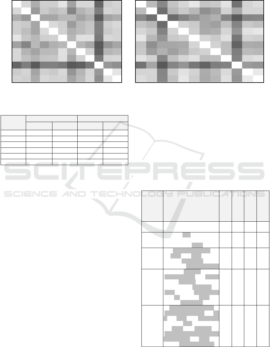
Table 2: Comparison of the calculated values of ν
C
i
C
j
for years 2008–2009 and 2013–2014.
ν
1 2 3 4 5 6
7 8 9 10 11
12
1 0.000 0.114 0.241 0.140 0.140 0.077
0.275 0.116 0.116 0.458 0.148
0.127
2 0.114 0.000 0.304 0.156 0.190 0.167
0.365 0.220 0.180 0.384 0.127
0.138
3 0.241 0.304 0.000 0.265 0.265 0.209
0.204 0.270 0.225 0.495 0.270
0.241
4 0.140 0.156 0.265 0.000 0.108 0.140
0.294 0.201 0.169 0.381 0.138
0.111
5 0.140 0.190 0.265 0.108 0.000 0.135
0.233 0.198 0.164 0.378 0.156
0.130
6 0.077 0.167 0.209 0.140 0.135 0.000
0.209 0.090 0.095 0.397 0.114
0.127
7 0.275 0.365 0.204 0.294 0.233 0.209
0.000 0.212 0.259 0.497 0.315
0.265
8 0.116 0.220 0.270 0.201 0.198 0.090
0.212 0.000 0.132 0.476 0.217
0.196
9 0.116 0.180 0.225 0.169 0.164 0.095
0.259 0.132 0.000 0.399 0.122
0.116
10 0.458 0.384 0.495 0.381 0.378 0.397
0.497 0.476 0.399 0.000 0.307
0.336
11 0.148 0.127 0.270 0.138 0.156 0.114
0.315 0.217 0.122 0.307 0.000
0.079
12 0.127 0.138 0.241 0.111 0.130 0.127
0.265 0.196 0.116 0.336 0.079
0.000
ν
1
2
3
4
5
6
7
8 9 10 11 12
1 0.000 0.220 0.386 0.188 0.132 0.077 0.185 0.172 0.090 0.452 0.138 0.111
2 0.220 0.000 0.466 0.228 0.172 0.228 0.362 0.317 0.146 0.286 0.135 0.138
3 0.386 0.466 0.000 0.476 0.405 0.344 0.286 0.251 0.394 0.537 0.394 0.389
4 0.188 0.228 0.476 0.000 0.143 0.169 0.283 0.307 0.201 0.397 0.175 0.198
5 0.132 0.172 0.405 0.143 0.000 0.153 0.272 0.259 0.135 0.341 0.098 0.079
6 0.077 0.228 0.344 0.169 0.153 0.000 0.135 0.169 0.101 0.439 0.143 0.159
7 0.185 0.362 0.286 0.283 0.272 0.135 0.000 0.146 0.209 0.505 0.267 0.275
8 0.172 0.317 0.251 0.307 0.259 0.169 0.146 0.000 0.206 0.415 0.217 0.233
9 0.090 0.146 0.394 0.201 0.135 0.101 0.209 0.206 0.000 0.405 0.119 0.101
10
0.452 0.286 0.537 0.397 0.341 0.439 0.505 0.415 0.405 0.000 0.328 0.344
11
0.138 0.135 0.394 0.175 0.098 0.143 0.267 0.217 0.119 0.328 0.000 0.071
12
0.111 0.138 0.389 0.198 0.079 0.159 0.275 0.233 0.101 0.344 0.071 0.000
Table 3: Maximal and minimal values of positive and
negative consonance between the twelve pillars of com-
petitiveness for years 2008–2009 to 2013–2014.
Year
µ ν
max(
µ
C
i
C
j
) min(
µ
C
i
C
j
) max(
ν
C
i
C
j
) min(
ν
C
i
C
j
)
2008–2009 0.860 0.389 0.497 0.077
2009–2010 0.865 0.410 0.505 0.071
2010–2011 0.852 0.447 0.468 0.087
2011–2012 0.870 0.405 0.534 0.074
2012–2013 0.870 0.421 0.519 0.071
2013–2014 0.873 0.399 0.537 0.071
From Table 3, we can make certain conclusions
about the range of values of the parameters α and β,
which are used to measure the consonance between
the criteria. Obviously, depending on how the values
of α and β have been chosen, different sets of
correlating criteria will form; and this can be done
over the data for each year. For the purposes of
illustration, let us only take the data for the latest
period (2013–2014), and check how the relations
between the criteria change by selecting different
values of α and β. Obviously, in this case putting
α > 0.873 or β < 0.071 would yield no results.
In general, the question how to select the values
of α and β, with respect to our various needs and
purposes, is important and challenging, but is
beyond the scope of the present research. Hence, we
will conduct our analysis by taking the following
exemplary pairs of (α; β): (0.85; 0.15), (0.80; 0.20),
(0.75; 0.25), (0.70; 0.30), (0.65; 0.35), and will see
which pillars are in positive consonance (Table 4,
those in negative consonance follow by analogy).
Obviously, values α = 0.85; β = 0.15 are rather
discriminative, since only two consonance pairs are
discovered to hold between four different criteria:
‘Institutions – Technological readiness’ and
‘Business sophistication – Innovation’, the second
one being quite natural, since these two pillars take
part in the formation of the ‘Innovation and
sophistication factors’ defining the difference
between the efficiency driven countries (2
nd
stage of
development) and innovation driven countries (3
rd
stage of development). The rest two criteria are of
more heterogeneous nature, where ‘Institutions’
belongs to the set of ‘Basic requirements’ and
‘Technological readiness’ belongs to the set of
‘Efficiency enhancers’.
Table 4: List of pillars in positive consonance for the year
2013–2014, per different α, β. Highlighted in grey on each
row are those consonances, which have been reported on
previous (upper) rows, the white ones appearing for first.
(α, β)
List of positive consonances
C
i
–C
j
No. of µ-pairs
No. of ν-pairs
No. of
consonances
No. of involved
criteria
(0.85;
0.15)
1–9; 11–12 2 19 2 4
(0.80; 0.2
0)
1–5; 1–6; 1–9; 1–11; 1–12; 2–
11; 5–11; 5–12; 9–11;
9–12; 11–12
11 29 11 7
(0.75; 0.2
5)
1–5; 1–6; 1–9; 1–11;
1–12; 2–9; 2–11; 2–12;
5–9; 5–11; 5–12; 6–9
6–11; 6–12; 9–11; 9–12; 11–1
2
17 37 17 7
(0.70;
0.30)
1–2; 1–4; 1–5; 1–6; 1–7; 1–8;
1–9; 1–11; 1–12; 2–5; 2–9; 2–
11; 2–12; 4–5;
4–11; 5–6; 5–9; 5–11;
5–12; 6–7; 6–8; 6–9; 6–11; 6–
12; 7–8; 8–9; 9–11;
9–12; 11–12
29 45 29 10
(0.65;
0.35)
1–2; 1–4; 1–5; 1–6; 1–7;
1–8; 1–9; 1–11; 1–12; 2–4; 2–
5; 2–6; 2–9; 2–10; 2–11; 2–12
;
3–8; 4–5; 4–6; 4–9;
4–11; 4–12; 5–6; 5–9;
5–11; 5–12; 6–7; 6–8; 6–9; 6–
11; 6–12; 7–8; 7–9; 8–9; 8–11
;
8–12; 9–11; 9–12; 11–12
39 51 39 12
Fourth International Symposium on Business Modeling and Software Design
292

The rest investigated values of α and β are
looser, thus yielding greater number of consonance
pairs between larger sets of criteria. We make the
detailed analysis only for the second pair, (0.8; 0.2).
Putting α > 0.8, we obtain 11 pairs of criteria
which have their µ > 0.8; and putting β < 0.2, we
obtain 29 pairs of criteria which have their ν < 0.2.
The first set of 11 pairs is completely a subset of the
second set of 29 pairs, meaning that we will discuss
only these 11 pairs, which are in positive conso-
nance; they connect 7 out of 12 pillars, as shown in
Table 5.
Table 5: List of pillars in positive consonance for the year
2013–2014, when α > 0.8, β < 0.2.
C
i
–C
j
Full titles of criteria C
i
–C
j
µ
C
i
C
j
ν
C
i
C
j
1–5
Institutions –
Higher education and training
0.807 0.132
1–6
Institutions –
Goods market efficiency
0.836 0.077
1–9
Institutions –
Technological readiness
0.854 0.090
1–11
Institutions –
Business sophistication
0.804 0.138
1–12
Institutions –
Innovation
0.844 0.111
2–11
Infrastructure –
Business sophistication
0.804 0.135
5–11
Higher education and training –
Business sophistication
0.815 0.098
5–12
Higher education and training –
Innovation
0.847 0.079
9–11
Technological readiness –
Business sophistication
0.810 0.119
9–12
Technological readiness –
Innovation
0.831 0.101
11–12
Business sophistication –
Innovation
0.873 0.071
Putting α = 0.75; β = 0.25, we obtain 17 pairs
w.r.t. α and 37 pairs w.r.t. β, giving a total of 17
pairs of consonance w.r.t. both parameters at a time.
In these 17 pairs take part again the same 7 criteria,
as in the previous case (0.80; 0.20), but 6 more
correlations between them are now discovered,
namely, ‘Infrastructure – Technological readiness’,
‘Infrastructure – Innovation’, ‘Higher education and
training – Technological readiness’, ‘Goods market
efficiency – Technological readiness’, ‘Goods mar-
ket efficiency – Business sophistication’ and ‘Goods
market efficiency – Innovation’.
The pairs (0.70; 0.30) and (0.65; 0.35) are rather
inclusive and non-discriminative values, since they
involve, respectively, 10 and 12 out of 12 pillars of
competitiveness and yield, respectively, 29 and 39
correlations between them.
We can visually illustrate the findings in Table 4
by constructing graphs for each run of α and β,
depicting the outlined dependences. We will do it
here only for the described case when α > 0.8,
β < 0.2, see Figure 1.
9
11
1
12
5
6
2
Figure 1: Graph structure of the pillars forming positive
consonance for the year 2013–2014 when α > 0.8, β < 0.2.
Now it becomes rather visual that when α > 0.8,
β < 0.2 three out of seven pillars completely correlate
with each other (‘1. Institutions’, ‘11. Business
sophistication’, ‘12. Innovation’), two other (‘5.
Higher education and training’ and ‘9. Technological
readiness’) completely correlate with the triple 1–11–
12, but not among each other, while vertices ‘2.
Infrastructure’ and ‘6. Good market efficiency’ are
connected by only one arc to the rest of the structure.
Obviously, for each run of α and β a series of
graphs will be formed, where every consequent
graph will act as a supergraph for the previous one,
becoming gradually more complex and intercom-
nected. It is interesting to compare for each run of α
and β whether and how these graph structures
change over the different time periods before 2013–
2014.
These graph structures are a matter of further
economic analysis, and it is particularly interesting
to study which of the pillars of competitiveness are
fully connected, like 1–5–11–12 and 1–9–11–12 in
Figure 1.
Also, it is noteworthy that in the WEF’s meth-
odology for forming the countries’ competitiveness
index, there are four sub-indicators take part in two
pillars each, namely: ‘Intellectual property pro-
tection’ takes part of the formation of the 1
st
and 12
th
pillar, ‘Mobile telephone subscriptions’ and ‘Fixed
telephone lines’ in 2
nd
and 9
th
pillar, and ‘Reliance
on professional management’ in 7
th
and 11
th
pillar.
We can hence make the conclusion, that our
findings generally support the proximity between the
mentioned pillars, as suggested by the presence of
shared sub-indicators, yet our conclusions are much
stronger and sophisticated as a result of the research.
It is also very important to make the comparison
Intercriteria Decision Making Approach to EU Member States Competitiveness Analysis
293

of the calculated values in Tables 1 and 2 between
years 2008–2009 and 2013–2014. We can focus the
reader’s attention to several particularly well
outlined observations. Over the period 2008–2014,
the pillars ‘5. Higher education and training’ and ‘7.
Labour market efficiency’ have become gradually
more correlated to all the rest pillars, while pillar ‘3.
Macroeconomic stability’ has become gradually less
correlated. However, in general, these comparisons
are a matter of detailed analysis by economists.
4 CONCLUSION
The present research aimed at discovery of some
hidden patterns in the data about EU Member States’
competitiveness in the period from 2008 to 2014.
We conduct the analysis of the World Economic
Forum’s Global Competitiveness Reports, using a
recently developed multicriteria decision making
method, based on index matrices and intuitionistic
fuzzy sets.
Using index matrices with data about how the
EU Member States have performed according to the
outlined twelve ‘pillars of competitiveness’, we
construct new matrices, giving us new knowledge
about how these pillars correlate and interact with
each other. Moreover, the application of the method
has been traced over a six-year period of time and
has revealed certain changes and trends in these
correlations that may yield fruitful further analyses
by interested economists. The results are illustrated
with data tables and graphs of the strongest cor-
relations between the criteria.
These conclusions may also be useful for the
national policy and decision makers, to better
identify and strengthen the transformative forces that
will drive their future economic growth. The same
approach can be equally applied to other selections
of countries and time periods, and comparisons with
the hitherto presented results will be challenging.
Besides the comparison of the twelve pillars of
competitiveness, our research plans include also
exploring the correlations between the most prob-
lematic factors for doing business, as outlined in the
WEF’s GCRs. Further investigation how the pillars
of competitiveness correlate with these most
problematic factors may also prove interesting and
useful.
ACKNOWLEDGEMENTS
The research work reported in the paper is partly
supported by the project AComIn “Advanced
Computing for Innovation”, grant 316087, funded
by the FP7 Capacity Programme (Research Potential
of Convergence Regions).
REFERENCES
Atanassov K. (1983) Intuitionistic fuzzy sets, VII ITKR's
Session, Sofia, June 1983 (in Bulgarian).
Atanassov K. (1986) Intuitionistic fuzzy sets. Fuzzy Sets
and Systems. Vol. 20 (1), pp. 87–96.
Atanassov K. (1991) Generalized Nets. World Scientific,
Singapore.
Atanassov K. (1999) Intuitionistic Fuzzy Sets: Theory and
Applications. Physica-Verlag, Heidelberg.
Atanassov K. (2012) On Intuitionistic Fuzzy Sets Theory.
Springer, Berlin.
Atanassov K., D. Mavrov, V. Atanassova (2013). Inter-
criteria decision making. A new approach for multi-
criteria decision making, based on index matrices and
intuitionistic fuzzy sets. Proc. of 12
th
International
Workshop on Intuitionistic Fuzzy Sets and General-
ized Nets, 11 Oct. 2013, Warsaw, Poland (in press).
World Economic Forum (2008, 2013). The Global
Competitiveness Reports. http://www.weforum.org/
issues/global-competitiveness.
Zadeh L. A. (1965). Fuzzy Sets. Information and Control
Vol. 8, pp. 333–353.
Fourth International Symposium on Business Modeling and Software Design
294