Using Nonlinear Models to Enhance Prediction Performance with

Incomplete Data

Faraj A. A. Bashir and Hua-Liang Wei

Department of Automatic Control and Systems Engineering, University of Shefﬁeld, Mapping Street, Shefﬁeld, U.K.

Keywords:

Missing Data, Maximum Likelihood, EM Algorithm, Gauss-Newton.

Abstract:

A great deal of recent methodological research on missing data analysis has focused on model parameter

estimation using modern statistical methods such as maximum likelihood and multiple imputation. These

approaches are better than traditional methods (for example listwise deletion and mean imputation methods).

These modern techniques can lead to unbiased parametric estimation in many particular application cases.

However, these methods do not work well in some cases especially for nonlinear systems that have highly

nonlinear behaviour. This paper explains the linear parametric estimation in existence of missing data, which

includes an overview of biased and unbiased linear parametric estimation with missing data, and provides

accessible descriptions of expectation maximization (EM) algorithm and Gauss-Newton method. In particular,

this paper proposes a Gauss-Newton iteration method for nonlinear parametric estimation in case of missing

data. Since Gauss-Newton method needs initial values that are hard to obtain in the presence of missing data,

the EM algorithm is thus used to estimate these initial values. In addition, we present two analysis examples

to illustrate the performance of the proposed methods.

1 INTRODUCTION

Missing data problems are closely related to statisti-

cal issues because most of missing data analysis and

design methods depend on statistical theory. In fact,

all predicted values for the missing data are depend-

ing on the probability functions. Some researchers

have considered missing data analysis problems to be

the most signiﬁcance issue in many real data analy-

ses and applications (Azar, 2002). More than often,

missing values are arbitrarily removed or simply re-

placed by mean values in simple missing data prob-

lems. This strategy, however, does not work well

for cases where there exist signiﬁcant missing val-

ues (Baraldi and Enders, 2010). Recent research has

concentrated on maximum likelihood methods such

as the EM (Expectation-Maximization) algorithm to

deal with missing data problems, which can produce

good results for most applications. Although this ap-

proach still has greater interest in the literature, es-

pecially in linear missing data analysis, there is no

enough knowledge to know if linear missing data

analysis methods can still give good result for non-

linear systems. Consequently, the overarching pur-

pose of this paper is to introduce some nonlinear

methods for missing data problems and to illustrate

the performance of nonlinear parametric estimation

by combining maximum likelihood estimation and a

Gauss-Newton iteration method. More speciﬁcally,

this article will present a brief overview of missing

data approaches, and provide accessible illustration of

expectation-maximization algorithm and the Gauss-

Newton optimization method. In some detail, we con-

centrate on Gauss-Newton iteration estimation and

present analysis examples.

2 MISSING DATA MECHANISMS

It is important to classify the mechanisms of miss-

ing data because this would determine which miss-

ing data handling strategies would be used for spe-

ciﬁc problems. There are three important patterns of

missing data which are MAR (missing at random),

MCAR (missing completely at random) and MNAR

(missing not at random) (Little and Rubin, 2002).

These patterns explain the relationships between the

inputs, and outputs of the system and the probabil-

ity density function of missing values. In more de-

tail, these mechanisms of missing values give the rea-

sons why these values are missing or unobserved. For

each pattern, a conceptual explanation will be given

141

A. A. Bashir F. and Wei H..

Using Nonlinear Models to Enhance Prediction Performance with Incomplete Data.

DOI: 10.5220/0005157201410148

In Proceedings of the International Conference on Pattern Recognition Applications and Methods (ICPRAM-2015), pages 141-148

ISBN: 978-989-758-076-5

 2015 SCITEPRESS (Science and Technology Publications, Lda.)

Table 1: The proportion of chlorine and length of time in

weeks with different missing data mechanism (Draper and

smith, 1981).

X Complete MAR MCAR MNAR

8 0.49 0.49 0.49 0.49

10 0.48 0.48 0.48 0.48

10 0.47 0.47 - 0.47

10 0.48 0.48 0.48 0.48

10 0.47 0.47 0.47 0.47

12 0.46 0.46 - 0.46

12 0.46 0.46 0.46 0.46

12 0.45 0.45 - 0.45

12 0.43 0.43 - 0.43

14 0.45 0.45 0.45 0.45

14 0.43 0.43 - 0.43

14 0.43 0.43 0.43 0.43

16 0.44 0.44 0.44 0.44

16 0.43 0.43 0.43 0.43

18 0.46 0.46 0.46 0.46

18 0.45 0.45 0.45 0.45

20 0.42 0.42 0.42 0.42

20 0.43 0.43 - 0.43

20 0.41 0.41 0.41 0.41

22 0.41 0.41 0.41 0.41

22 0.40 0.40 0.4 -

22 0.42 0.42 0.42 0.42

24 0.40 0.40 - -

24 0.40 0.40 0.40 -

24 0.41 0.41 - 0.41

26 0.40 0.40 0.4 -

26 0.41 0.41 0.41 0.41

28 0.40 0.40 0.40 -

30 0.40 - - -

30 0.38 - 0.38 0.38

30 0.41 - 0.41 0.41

32 0.40 - - -

32 0.40 - 0.40 -

34 0.40 - 0.40 -

36 0.41 - 0.41 0.41

36 0.38 - - 0.38

38 0.40 - 0.40 -

40 0.39 - 0.39 0.39

42 0.39 - 0.39 0.39

in the next paragraph, and for more details on miss-

ing data mechanisms, see (Graham, 2009; Schlomer

et al., 2010).

Values are missing at random (MAR) when the

probability of a missing value on an output Y (vari-

able Y) is related to the input (or inputs) U in the

system but not to the response of the output Y itself.

In other words, the probability of the missing values

depends on the relation between the output Y and in-

put (or inputs) U, that means there is no direct rela-

tionship between the probability of the missing val-

ues on Y and the values of Y variable itself. Data are

missing completely at random (MCAR) is a mecha-

nism where the probability of a missing value in Y

does not depend on the output Y and the input (or in-

puts) U. Values are missing not at random (MNAR),

if the probability of incomplete value on an output Y

depends on Y itself but not on the input (or inputs)

U. That means the probability of the missing values

dont have relation between the output Y and input (or

inputs) U (Schafer and Graham, 2002).To give more

detail, let have a look at the data given in Table.1,

which was taken from (Draper and Smith, 1981). In

this example, the dependent variable (Y) is the pro-

portion of available chlorine in a certain quantity of

chlorine solution and the independent variable (X) is

the length of time in weeks since the product was pro-

duced. When the product is produced, the proportion

of chlorine is 0.50. During the 8 weeks that it takes to

reach the consumer, the proportion declines to 0.49.

The ﬁrst two columns in Table.1 show the com-

plete values for two variables (input X and output Y).

The remaining columns represent the amount of Y,

which appear in hypothetical missed data by three

mechanisms. In the third column, the probability

of missing values has a direct relationship with the

variable X where the values started missing after 30

weeks (X > 28), this mechanism is MAR. In the

second case, there are 11 measured values randomly

selected from those measured in 42 weeks; which

means that the probability of each missing data is not

affected by the value of X and the values of Y vari-

able itself, that means the mechanism is MCAR but

not MAR. In the ﬁfth column, those equal to 0.40 (Y

= 0.40) were unobserved, and for these values there

is no direct relation between the input variable X and

the output Y. In other words, the probability of miss-

ing values depends on the variable Y only. This third

case represents of MNAR.

3 TRADITIONAL MISSING-DATA

TECHNIQUES

Many missing data analysis methods have been pre-

sented in the literature. In this paper, we describe a

limited selection of these approaches. Readers are re-

ferred to (Schafer and Graham, 2002; Enders, 2010)

for detailed information on missing data.

ICPRAM2015-InternationalConferenceonPatternRecognitionApplicationsandMethods

142

3.1 Listwise Deletion

Listwise deletion throws away data whose informa-

tion is insufﬁcient. Listwise deletion is also known

as Filtering Approaches and complete-case analysis

(CDS). This method is used in many missing data

problems, but its implementation depends on the type

of data mechanism (Baraldi and Enders, 2010). That

means CDS pays attention to data that have observed

values only. For example, if we are calculating a mean

and variance for variable Y, CDS discards any cases,

which have missing values on the variable Y, those

omitted values may lead to biased parametric estima-

tion (Allison, 2002). On the other hand, by omitting

the missing values it has a direct dramatic reduction in

the complete data. When data missing is completely

at random this technique would then generate unbi-

ased estimation but with large number of removed

data this is not true (Enders and Bandalos, 2001).

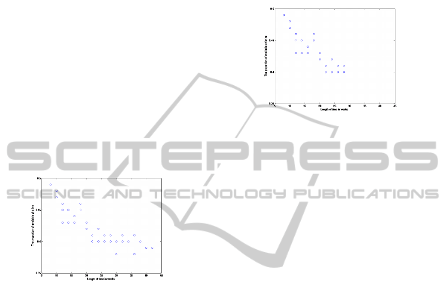
Figure 1: Complete-data scatterplot of the proportion of

available chlorine in a certain quantity of chlorine solution.

To explain the principles of deletion approach, the

data set in Table.1 for the proportion of available chlo-

rine and length of time in weeks are taken as an ex-

ample. Fig.1 shows a scatterplot of the complete cases

because there are only two variables; the negative cor-

relation between the input X and the output Y (-0.86)

means that the low proportion of available chlorine

would have acquired high length of time in weeks.

Fig.2 shows a scatterplot of the deletion approaches

in case of MAR, we will focus on this mechanism to

show the effect of the bias on these approaches. Be-

cause listwise deletion takes the observed data of the

variable Y, it systematically ignores values from 28

weeks. The plot also shows that there is weak non-

linear variation and association between Y and X. In

case of complete data set, the estimated value of the

variable Y (mean value) is 0.425, whereas the case

of omitted data analysis gives an estimated value of

0.435. Similarly, the estimated value of the variable X

is 22.27 and 17.56 for the complete-data and listwise

deletion, respectively. Even with taking the standard

deviation into consideration, the proportion of avail-

able chlorine have a standard deviation 0.03053 in the

complete case, in contrast the listwise deletion gives a

standard deviation 0.02907 that means there is atten-

uation in the system.

Figure 2: Listwise deletion scatterplot of the proportion of

available chlorine in a certain quantity of chlorine solution

(MAR).

3.2 Imputation Methods

Imputation points to a group of common traditional

missing data methods where the estimator imputes

(changes) the missing values with appropriate values

(Little and Rubin, 2002). In fact, there are many im-

putation approaches. This study will concentrate on

three of the most common methods: mean substi-

tution imputation, linear regression imputation, and

stochastic (random) regression imputation. The sim-

plest one is mean imputation method, which imputes

the missing values with the mean of the observed

data (Enders, 2006; Allison, 2002). For example for

the data in Table.1 for the MAR mechanism case the

expected value of the observed output is 0.435, this

value can represent the missing values in all cases.

Fig.3 shows that the estimated data from mean substi-

tution imputation are in straight line cross the Y-axis

at 0.435 and has a zero slope. In this case the correla-

tion between the input X and the output Y is equal to

zero and this is because the imputation of the missing

data depending only on the output Y. With focusing

on more features of mean imputation method, cross

correlation between the imputed output and input X

is -0.497, in contrast the complete-data correlation is

-0.86 (the negative sign represent the opposite rela-

tion between the input and the output as the input in-

crease the output decrease). The data variability may

not appear when the missing values are replaced by

the average of observed data (a constant value). With

taking the mean and standard deviation in consider-

ation, the mean imputation produces mean and stan-

dard deviation 0.435 and 0.025 respectively, meaning

that there is attenuation in the system. Regression im-

putation is a technique that ﬁlls missing values with

UsingNonlinearModelstoEnhancePredictionPerformancewithIncompleteData

143

expected value by using a regression model (Schafer,

2010). In this method, observed data of the output Y

are used to estimate a regression model, which is used

to predict the value of missing data. Again, take the

data in Table.1 as an example. In MAR mechanism,

there are 12 unobserved values and 32 observed cases.

The observed data of output Y (variable with missing

data) are used with observed data on input X (vari-

able with complete data) to estimate the missing cases

on output Y. In this case we have used linear regres-

sion model:

Y = 0.509 − .0042X. Applying the input

X (complete data) on the regression model yields pre-

dicted output (

Y ), and these predicted data represents

the missing data of the output Y in the system.

Figure 3: Mean imputation scatterplot of the proportion of

available chlorine in a certain quantity of chlorine solution

(MAR).

The basic idea of the regression imputation de-

pends on a technique of borrowing information from

the observed data from the output variable, this

method also leads to biased estimation, as shown in

Fig.4. Notice that the estimated missing data repre-

sents a straight line with a slope of - 0.0042. This

means that the output of the system with imputed data

has maximum correlation value (corr=1.0 between the

imputed output

Y and input X). Notice that the linear

regression imputation yields a correlation equal to -

0.97 between the output Y and input X, in contrast

with the correlation of -0.86 for the complete-data.

Because the imputed data are generated by a linear

function, there are no ﬂuctuations for the estimated

values. Consequently, the imputation process will at-

tenuate the variability of the estimation data. For ex-

ample, the standard deviation of output Y from lin-

ear regression estimation is 0.042, whereas it is equal

to 0.025 in case of complete data. Although linear

imputation gives biased estimation of standard devia-

tion and correlation for the data mechanism MCAR or

MAR, it does yield unbiased estimates of the average.

Mean substitution imputation and linear impu-

tation lead to bias estimation, especially in case

of correlation and standard deviation of both MAR

and MCAR (Allison, 2002; Graham, 2009; Schafer,

Figure 4: Regression model scatterplot of the proportion of

available chlorine in a certain quantity of chlorine solution

(MAR).

2010). Stochastic linear regression imputation can

eliminate these missing values, it is similar to stan-

dard regression imputation technique and a regres-

sion model estimates for the missing data (Baraldi

and Enders, 2010). In some detail, it is a linear re-

gression imputation with each estimated value being

added a random error value; this random value is gen-

erated randomly from a normal distribution with a

variance equal to the residual variance and a mean

of zero that is estimated from the linear regression

imputation model (Schafer, 2010; Graham, 2009).

Recall the data in Table.1, where the regression of

the output Y on input X yield a residual variance of

0.000162. Then, the new random error is produced

randomly from a normal distribution with a variance

of 0.000162 and a mean of zero. These new error

terms can then be added to the estimated output

Y ,

which is predicted from the linear regression impu-

tation model. Fig.5 shows the scatter plot of the im-

puted values of available chlorine data obtained from

a stochastic linear imputation model. Because there

is a random error added to each imputed value the

imputed data do not represent a straight line, as that

generated from a standard linear regression imputa-

tion model.

Figure 5: Stochastic imputation scatterplot of the propor-

tion of available chlorine in a certain quantity of chlorine

solution (MAR).

Comparing Fig.1 with Fig.5, it is clear that the

ICPRAM2015-InternationalConferenceonPatternRecognitionApplicationsandMethods

144

stochastic regression model produces much better re-

sult. This slight adjustment to regression model yields

unbiased parameter estimation in the case of MAR

mechanises. However, stochastic regression imputa-

tion may not be able to guess the real error between

the real and predicted values because it depends on

random error values.

4 EM ALGORITHM

EM algorithm is an iterative technique, which is use-

ful for incomplete data analyses, and it is an algo-

rithm depending on a maximum likelihood technique

to produce a group of data by using the relationships

among all observed variables(Enders, 2010). The ba-

sic idea of this technique was developed in 1970s

(Dempster et al., 1977). This algorithm consists of it-

erative procedures, which are divided into two steps,

that is the expectation step and the maximization step

(E and M steps, respectively). As an iterative algo-

rithm it needs initial values to start, these initial values

are represented by a mean vector and covariance ma-

trix. To generate the initial values of the mean vector

and the covariance matrix we can use much simple

technique such as listwise deletion method (Enders,

2010). EM technique uses linear regression models

to estimate the missing data and sometimes gives bi-

ased estimation especially when the system contains

high nonlinearity behaviour (Smyth, 2002; Ng et al.,

2012). This study proposes a modiﬁed iterative al-

gorithm to deal with nonlinear system models, where

there exist a number of latent variables. It follows

that for small data set problems, the EM algorithm

gives the same result as regression imputation tech-

nique (Baraldi and Enders, 2010).

5 NONLINEAR ESTIMATION BY

GAUSS-NEWTON ALGORITHM

The linearization technique for nonlinear regression

is an approach widely used in nonlinear regression

model estimation (Montgomery et al., 2006). The

basic idea of nonlinear estimation by linearization

method consists of two steps, that is the linearization

of the nonlinear system and the estimation of model

parameters (Smyth, 2002). Linearization can be im-

plemented by a Taylor series expansion of the nonlin-

ear model regarding a speciﬁc operating point. For

example for a nonlinear model f (X,β) of n parame-

ters (X is input and β is the estimated parameter vec-

tor) the linearization result with respect to the opera-

tion point β

f (X

,β) = f (X

,β

) +

∑

m=1



∂ f (X

,β)

∂β



β=β

(β

− β

)

(1)

= f (X

,β

) (2)

= (β

− β

) (3)

∂ f (X

,β)

∂β

β=β

is k ×n jacobian matrix. The

residual between linear and nonlinear values for the

nonlinear model is

e = Y

− f

∑

m=1

+ ε

(4)

The linear model (3) is assumed to be valid just

around some speciﬁc operating point and ε is assumed

to be white noise with zero mean and constant vari-

ance. Least squares method can be used to estimate

parameter α

= J

+ ε (5)





−1

e (6)

From equation (1),

= α

+ β

(7)

The next step is to replace β

by β

in equation

(1) which represents new initial value for the sys-

tem and repeat same steps for [β

,β

,.........,β

]

where l is the number of required iterations to get

the convergence. We can calculate the number of

iterations m by determining the convergence ratio

([(α

k,l+1

− α

)/α

]) < δ at each iteration until it

meets some pre-speciﬁed threshold (speciﬁc small

value for δ) for example when the value less than

1 × 10

−6

(Montgomery et al., 2006). The above pro-

cedures are called Gauss-Newton iteration method for

nonlinear system analysis. Unfortunately, this tech-

nique cannot be used to estimate the parameters if

there exist missing data because it depends on the

error between the linear and nonlinear values and if

there is a missing value on the output Y it is not pos-

sible to estimate the error. This study thus tries to

use another optimization technique (that is the EM al-

gorithm) to estimate the error and take it as an ini-

tial value in the Gauss-Newton iteration approach. It

shows that the combination of EM and Gauss-Newton

approach produces better results in comparison with

linear analysis methods. To illustrate this, the same

example taken from (Draper and Smith, 1981)was

considered here.

UsingNonlinearModelstoEnhancePredictionPerformancewithIncompleteData

145

Figure 6: Nonlinear scatterplot of the proportion of avail-

able chlorine in a certain quantity of chlorine solution

(MAR).

Firstly, a nonlinear exponential growth model is

used to ﬁt the data

Y = θ

− θ

(X−x

)

(8)

where x

and y

represent the ﬁrst two values in

the data set (initial values). The values generated by

the estimated nonlinear model are shown in Fig.6.

Comparing Fig.6 with Fig.4 and Fig.5, there is sim-

ilarity between the linear estimation and the nonlin-

ear estimation. This slight modiﬁcation to nonlinear

algorithm for missing data yields unbiased parame-

ter estimation in the MAR case. Notice that the non-

linear regression model yields a correlation -0.94 be-

tween the output Y and input X, in contrast the cor-

relation equals to -0.86 for the complete-data. Conse-

quently, the nonlinear model produces less variability,

for example, the standard deviation of the output Y

estimated from the nonlinear model is 0.029, whereas

it is equal to 0.025 for the complete data. Although

nonlinear regression model gives unbiased estimation

of standard deviation and correlation, it does produce

biased estimate of the mean. In the above example,

an exponential growth model was used to ﬁt the data,

which shows some disadvantage in comparison with

linear models. Next, it presents the use of EM algo-

rithm for linear model parameter estimation, and the

use of the modiﬁed Gauss-Newton algorithm nonlin-

ear model parameter estimation. (Enders, 2006; Gra-

ham, 2009; Schlomer et al., 2010; Seaman and White,

2013; Montez-Rath et al., 2014). To give more de-

tails let us consider another data set which is taken

from (Montgomery et al., 2006), and shown in Ta-

ble.2. In this example, the dependent variable (Y) is

the tensile strength of Kraft paper and the independent

variable (X) is the hardwood concentration for pulp,

which produces the paper. The data set in this exam-

ple contains complete data on the input and output of

the system. The data set also includes the following

missing data mechanism: data missing completely at

random (MCAR) with 21%, 26% and 37% missing.

Note that unlike in the previous examples, the choice

of this mechanism is to study the effect of different al-

gorithms on different missing mechanisms. The ulti-

mate purpose of this example is to compare the perfor-

mance of linear algorithm (EM algorithm) and nonlin-

ear algorithm (modiﬁed Gauss-Newton algorithm) in

the presence of different percentages of missing data

for a MCAR mechanism in term of correlations, resid-

uals, standard deviations, and means. For illustration,

the complete data are plotted in Fig.7. The EM al-

gorithm is applied to estimate the parameters of the

linear model:

Y = θ

+ θ

X (9)

Figure 7: NComplete data scatterplot of input/output data.

The modiﬁed Gauss-Newton algorithm was ap-

plied to estimate the parameters of the nonlinear

model:

Y = θ

+ θ

X +θ

(10)

Let us start by comparing the estimated values gen-

erated by the linear and nonlinear models (in case of

MCAR with 21% missing data ), with that of the com-

plete data, where the mean value for full-observed

output Y is 34.184, and mean value for the predicted

values is 34.379, and 34.178, respectively. This result

indicates that the nonlinear regression is just slightly

better than the linear model for mean value estima-

tion. By inspecting Fig.8 and Fig.9, it can be seen

that the effect of linear regression on the system. In

Fig.8, the predicted values from linear model fall di-

rectly on a straight line that has a slope 1.73, the same

thing happens with the nonlinear model in Fig.9. The

predicted values with linear and nonlinear regression

have a correlation 0.54684 and 0.53117 respectively

between the predicted output and input X, whereas

the case of complete data has a correlation 0.55261.

Table.3, summarises the effect of other two cases of

percentage missing (MCAR 26% and MCAR 37%)

on the linear and nonlinear model. For example, lin-

ear and nonlinear model give standard deviation esti-

mates of 13.61 and 14.00, respectively, whereas the

full-observed data standard deviation is 13.778. Not

surprisingly, this is because the missing values are

close to linear region area.

ICPRAM2015-InternationalConferenceonPatternRecognitionApplicationsandMethods

146

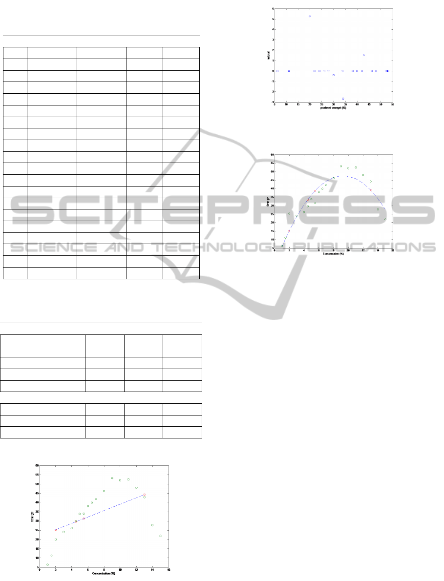
Table 2: The input and output of the system in MCAR

with missing percentage (Montgomery et al., 2006) (Mont-

gomery, Peck,and Vining, 2006).

Y-MCAR

X Complete (21%) (26%) (37%)

1 6.3 6.3 6.3 6.3

1.5 11.1 11.1 11.1 11.1

2 20 - 20 -

3 24 24 24 24

4 26.1 26.1 26.1 26.1

4.5 30 - - -

5 33.8 33.8 33.8 33.8

5.5 34 - 34 -

6 38.1 38.1 - 38.1

6.5 39.9 39.9 39.9 -

7 42 42 - 42

8 46.1 46.1 46.1 -

9 53.1 53.1 53.1 -

10 52 52 - 52

11 52.5 52.5 52.5 52.5

12 48 48 - -

13 42.8 - 42.8 42.8

14 27.8 27.8 27.8 27.8

15 21.9 21.9 21.9 21.9

Table 3: The effect of linear and nonlinear models on the

system in different MCAR missing percentage.

Linear regression

21% 26% 37%

Mean 34.379 31.744 31.106

Correlation 0.5468 0.543 0.5541

Standard deviation 13.61 13.778 13.778

Nonlinear regression

Mean 34.178 30.945 31.426

Correlation 0.5312 0.5148 0.5372

Standard deviation 14.01 12.438 12.356

Figure 8: Linear regression model of input/output data in

case of 21% missing data scatter plot.

Figure 9: Linear regression model residual e versus pre-

dicted values scatter plot in case of 21% missing.

Figure 10: Nonlinear regression model of input/output data

in case of 21% missing data scatter plot.

6 CONCLUSIONS AND FUTURE

WORK

The primary aim of this paper is to introduce a non-

linear modelling technique for missing-data analy-

sis. Comparative studies on EM and Gauss-Newton

approaches have been carried out. EM and Gauss-

Newton algorithms are advantageous over traditional

approaches. Although EM and Gauss-Newton algo-

rithms have not produced same results specially in

existing of high nonlinearity in the system and dif-

ferent missing data mechanism (i.e., MAR and dif-

ferent MCAR cases). Most studies in the literature

focus on using of linear techniques because they hold

the simplest assumptions that make these procedures

easier for users especially in computerised environ-

ment. As mentioned previously, in existence of high

nonlinearity parts in the system, EM does not always

give good result. Although Gauss-Newton does need

initial values to start iteration process and that gives

it disadvantage because this needs more time to do

in computerised environment. In summary, EM and

Gauss-Newton algorithms require similar procedures

and frequently produce similar parameter estimates

(in case of small number of data for both MAR and

MCAR mechanism), particularly if the distribution of

data contains low nonlinear parts. As a future work,

UsingNonlinearModelstoEnhancePredictionPerformancewithIncompleteData

147

for a nonlinear model, the form of the model must be

speciﬁed, the parameters need to be estimated, and

starting values for those parameters must be carefully

provided.(Box and Tidwell, 1962) proposed the ﬁrst

technique for model selection. (Royston and Sauer-

brei, 2008) suggested a class of regression models by

fractional polynomials (FP), involving model choice

from a speciﬁc number of models, but all of these

methods work only in case of complete data. We will

try to modify one of these approaches and apply it on

missing data. To further improve and test the perfor-

mance of the proposed method, we will try and incor-

porate good ideas of other methods for example those

presented in (Luengo et al., 2012)also carry out com-

parative studies on real data sets, readers are referred

to (Alcal

a et al., 2010) for good sample data sets.

REFERENCES

Alcal

a, J., Fern

andez, A., Luengo, J., Derrac, J., Garc

ıa,

S., S

anchez, L., and Herrera, F. (2010). Keel data-

mining software tool: Data set repository, integration

of algorithms and experimental analysis framework.

Journal of Multiple-Valued Logic and Soft Computing,

17:255–287.

Allison, P. D. (2002). Missing data: Quantitative applica-

tions in the social sciences. British Journal of Mathe-

matical and Statistical Psychology, 55(1):193–196.

Azar, B. (2002). Finding a solution for missing data. Mon-

itor on Psychology, 33(7):70–1.

Baraldi, A. N. and Enders, C. K. (2010). An introduction

to modern missing data analyses. Journal of School

Psychology, 48(1):5–37.

Box, G. E. and Tidwell, P. W. (1962). Transformation of the

independent variables. Technometrics, 4(4):531–550.

Dempster, A. P., Laird, N. M., and Rubin, D. B. (1977).

Maximum likelihood from incomplete data via the em

algorithm. Journal of the Royal Statistical Society. Se-

ries B (Methodological), pages 1–38.

Draper, N. R. and Smith, H. (1981). Applied regression

analysis 2nd ed.

Enders, C. K. (2006). A primer on the use of modern

missing-data methods in psychosomatic medicine re-

search. Psychosomatic medicine, 68(3):427–436.

Enders, C. K. (2010). Applied missing data analysis. Guil-

ford Press.

Enders, C. K. and Bandalos, D. L. (2001). The relative per-

formance of full information maximum likelihood es-

timation for missing data in structural equation mod-

els. Structural Equation Modeling, 8(3):430–457.

Graham, J. W. (2009). Missing data analysis: Making it

work in the real world. Annual review of psychology,

60:549–576.

Little, R. J. and Rubin, D. B. (2002). Statistical analysis

with missing data.

Luengo, J., Garc

ıa, S., and Herrera, F. (2012). On the

choice of the best imputation methods for missing val-

ues considering three groups of classiﬁcation meth-

ods. Knowledge and information systems, 32(1):77–

108.

Montez-Rath, M. E., Winkelmayer, W. C., and Desai, M.

(2014). Addressing missing data in clinical studies

of kidney diseases. Clinical Journal of the American

Society of Nephrology, pages CJN–10141013.

Montgomery, D., Peck, E., and Vining, G. (2006). Diagnos-

tics for leverage and inﬂuence: Introduction to linear

regression analysis . hoboken.

Ng, S. K., Krishnan, T., and McLachlan, G. J. (2012). The

em algorithm. In Handbook of computational statis-

tics, pages 139–172. Springer.

Royston, P. and Sauerbrei, W. (2008). Multivariable model-

building: a pragmatic approach to regression anaylsis

based on fractional polynomials for modelling contin-

uous variables, volume 777. John Wiley & Sons.

Schafer, J. L. (2010). Analysis of incomplete multivariate

data. CRC press.

Schafer, J. L. and Graham, J. W. (2002). Missing data: our

view of the state of the art. Psychological methods,

7(2):147.

Schlomer, G. L., Bauman, S., and Card, N. A. (2010). Best

practices for missing data management in counsel-

ing psychology. Journal of Counseling Psychology,

57(1):1.

Seaman, S. R. and White, I. R. (2013). Review of inverse

probability weighting for dealing with missing data.

Statistical Methods in Medical Research, 22(3):278–

295.

Smyth, G. K. (2002). Nonlinear regression. Encyclopedia

of environmetrics.

ICPRAM2015-InternationalConferenceonPatternRecognitionApplicationsandMethods

148